2.7 Rules Depending on More Than One Relation

A crucial simplifying feature of the rules we have considered so far is that they depend only on one relation, so that in a collection of relations, the rule can be applied separately to each relation (cf. [1:p82]). Put another way, this means that all the rules we have considered always transform single edges or hyperedges independently.

But consider a rule like:

This can be represented graphically as:

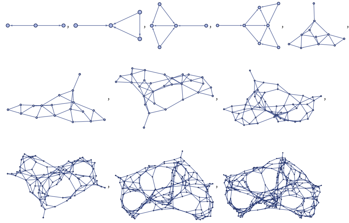
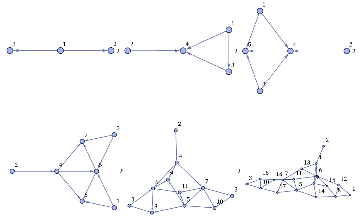
Here is the result of running the rule for several steps:

Here is the result for 10 steps:

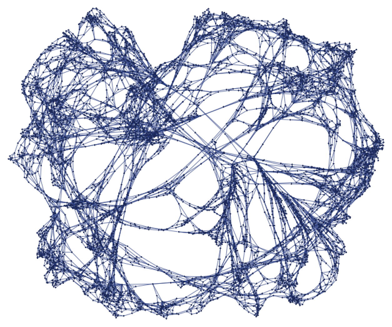
Despite the simplicity of the underlying rule, the structure that is built (here after 15 steps, and involving 6974 elements and 13,944 relations) is complex:

In getting this result, we are, however, glossing over an important issue that will occupy us extensively in later sections, and that potentially seems intimately connected with foundational features of physics.

With a rule that just depends on a single relation, there is in a sense never any ambiguity in where the rule should be applied: it can always separately be used on any relation. But with a rule that depends on multiple relations, ambiguity is possible.

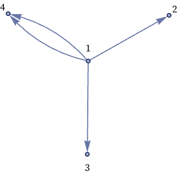
Consider the configuration:

The rule

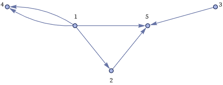
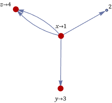
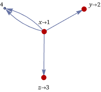
can be applied here in two distinct, but overlapping, ways. First, one can take

giving the result:

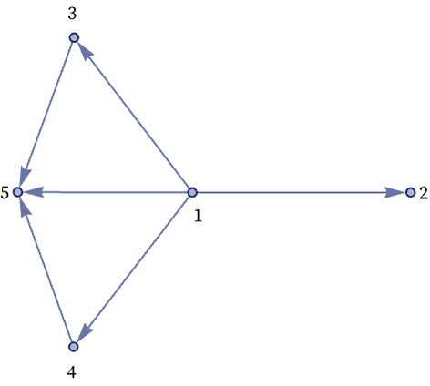
But one can equally well take

giving the inequivalent result:

With a rule that just depends on a single relation, there is an obvious way to define a single complete step in the evolution of the system: just make it correspond to the result of applying the rule once to each relation. But when the rule involves multiple relations, we have seen that there can be ambiguity in how it is applied (cf. [1:p501]), and one consequence of this is that there is no longer an obvious unique way to define a single complete step of evolution. For our purposes at this point, however, we will take each step to be what is obtained by scanning the configuration of the system, and finding the largest number of non-overlapping updates that can be made (cf. [1:p487]). In other words, in a single step, we update as many edges (or hyperedges) as possible, while never updating any edge more than once.

For now, this will give us a good indication of what kind of typical behavior different rules can produce. Later, we will study the results of all possible updating orders. And while this will not affect our basic conclusions about typical behavior, it will have many important consequences for our understanding of the models presented here, and their potential relevance to fundamental physics.