There are many graph and hypergraph properties that can be studied for the output of our models. Here we primarily give examples for the rule {{x,y},{x,z}}{{x,z},{x,w},{y,w},{z,w}} discussed above.
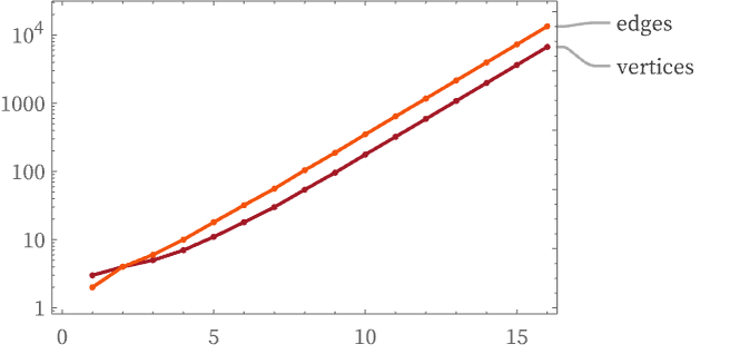
A basic question is how the numbers of vertices and edges (elements and relations) grow with successive steps. Plotting on a logarithmic scale suggests eventually roughly exponential growth in this case:
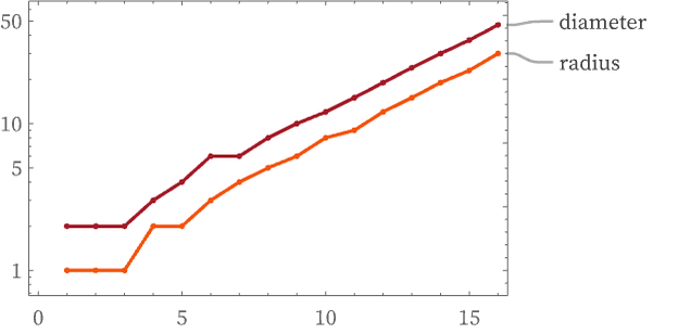
We can also compute the growth of the graph diameter (greatest distance between vertices) and graph radius:
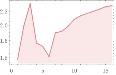
If one assumes that the total vertex count V is related to diameter D by V = Dd, then plotting d gives (to be compared to dimension approaching ≈2.68 computed from the growth of Vr):
There are many measures of graph structure which basically support the expectation that after many steps, the outputs from the model somehow converge to a kind of statistically invariant “equilibrium” state:

Some centrality measures [32][33] start (here at step 10) somewhat concentrated, but rapidly diffuse to be much more broadly distributed:

There are local features of the graph that are closely related to V1(X) and V2(X):

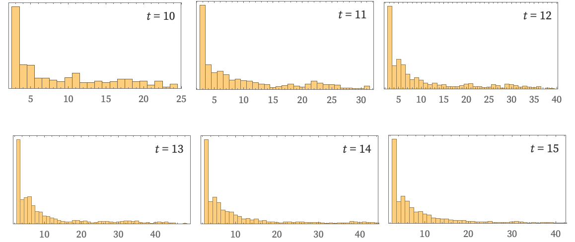
Another feature of our graphs to study is their cycle structure. At the outset, our graphs give us only connectivity information. But one way to imagine identifying “faces” that could be used to infer emergent topology is to look at the fundamental cycles in the graph:
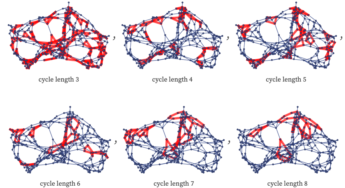
In this particular graph, there are altogether 320 fundamental cycles, with the longest one being of length 24. The distribution of cycle lengths on successive steps once again seems to approach an “equilibrium” form:
One way to probe overall properties of a graph is to consider the evolution of some dynamical process on the graph. For example, one could run a totalistic cellular automaton with values at nodes of the graph. Another possibility is to solve a discretized PDE. For example, having computed a graph Laplacian [34] (or its higher order analogs) one can determine the distribution of eigenvalues, or the eigenmodes, for a particular graph [35]. The density of eigenvalues is then closely related to Vr and our estimates of dimension and curvature.
 download pdf
  ARXIV
ARXIV peer review