 download pdf
  ARXIV
ARXIV peer review
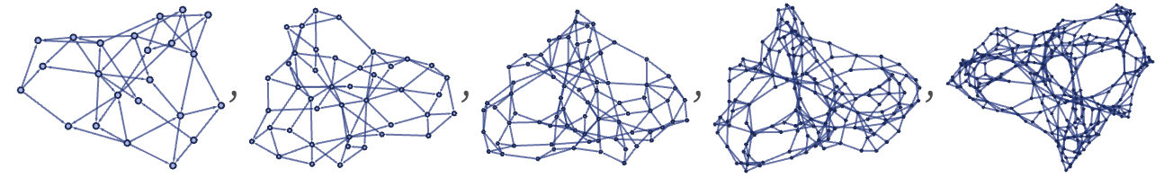
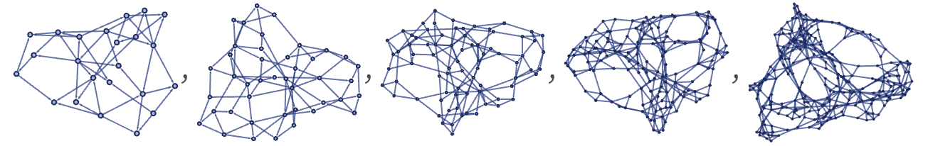
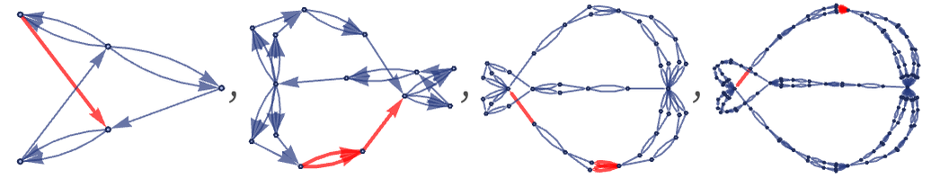
Imagine that at some step in the evolution of a rule one reverses a single relation. What effect will it have? Here is an example for the rule {{x,y},{x,z}}{{x,z},{x,w},{y,w},{z,w}}. The first row is the original evolution; the second is the evolution after reversing the relation:
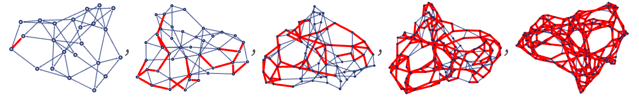
We can illustrate the effect by coloring edges in the first row of graphs that are different in the second one (taking account of graph isomorphism) [41]:
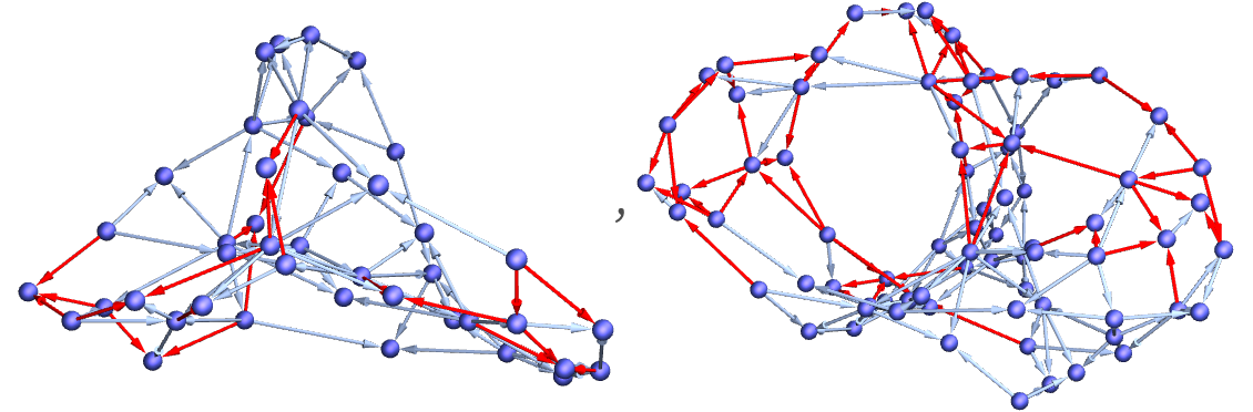
Visualizing the second and third graphs in 3D makes it more obvious that the changed edges are mostly connected:
It takes only a few steps before the effect of the change has spread to essentially all parts of the system. (In this particular case, with the updating order used, about 20% of edges are still unaffected after 5 steps, with the fraction slowly decreasing, even as the number of new edges increases.)
In rules with fairly simple behavior, it is common for changes to remain localized:
However, when complex behavior occurs, changes tend to spread. This is analogous to what is seen, for example, in the much simpler case of class 2 versus class 3 cellular automata [31][1:6.3]:
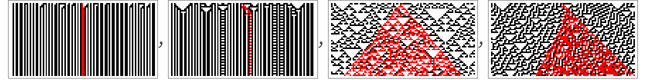
Cellular automata are also known [31] to exhibit the important phenomenon of class 4 behavior—in which there is a discrete set of localized “particle-like” structures through which changes typically propagate:
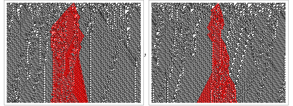
In cellular automata, there is a fixed lattice on which local rules operate, making it straightforward [1:6.3] to identify the region that can in principle be affected by a change in initial conditions. In the models here, however, everything is dynamic, and so even the question of what parts can in principle be affected by a change in initial conditions is nontrivial.
As we will discuss at length later, however, it is always possible to trace which updating events in a particular evolution depend on which others, and which relations are associated with these. The result will always be a superset of the actual effect of a change in the initial condition:
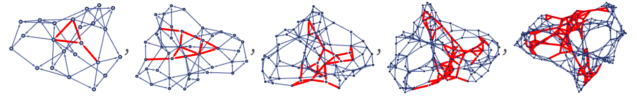
We discussed above the quantity Vr(X) obtained by “statically” looking at the number of nodes in a hypergraph reached by going graph distance r—in effect computing the volume of a ball of radius r in the hypergraph. By looking at the dependence of updating events in t successive steps of evolution, we can define another quantity Ct(X) which in effect measures the volume of a cone of dependencies in the evolution of the system.
Vr(X) is in a sense a quantity that is “applied” to the system from outside; Ct(X) is in a sense intrinsic. But as we will discuss later, Vr(X) is in some sense an approximation to Ct(X)—and particularly when we can reasonably consider the evolution of a model to have reached some kind of “equilibrium”, Vr(X) will provide a useful characterization of the “state” of a model.