The Notion of Dimension: Wolfram Physics Project Technical Background

In traditional geometry, a basic feature of any continuous space is its dimension. And we have seen that at least in certain cases we can characterize the limiting behavior of our models in terms of the emergence of recognizable geometry—with definite dimension. So this suggests that perhaps we might be able to use a notion of dimension to characterize the limiting behavior of our models even when we do not readily recognize traditional geometrical structure in them.

For standard continuous spaces it is straightforward to define dimension, normally in terms of the number of coordinates needed to specify a position. If we make a discrete approximation to a continuous space, say with a progressively finer grid, we can still identify dimension in terms of the number of coordinates on the grid. But now imagine we only have a connectivity graph for a grid. Can we deduce what dimension it corresponds to?

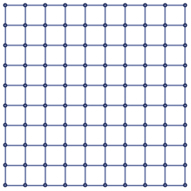
We might choose to draw the grids so they lay out according to coordinates, here in 1-, 2- and 3-dimensional Euclidean space:

GridGraph[{10}, VertexStyle -> ResourceFunction["WolframPhysicsProjectStyleData"]["SpatialGraph", "VertexStyle"], EdgeStyle -> ResourceFunction["WolframPhysicsProjectStyleData"]["SpatialGraph", "EdgeLineStyle"]]

GridGraph[{10, 10}, VertexStyle -> ResourceFunction["WolframPhysicsProjectStyleData"]["SpatialGraph", "VertexStyle"], EdgeStyle -> ResourceFunction["WolframPhysicsProjectStyleData"]["SpatialGraph", "EdgeLineStyle"]]

GridGraph[{5, 5, 5}, VertexStyle -> ResourceFunction["WolframPhysicsProjectStyleData"]["SpatialGraph", "VertexStyle"], EdgeStyle -> ResourceFunction["WolframPhysicsProjectStyleData"]["SpatialGraph", "EdgeLineStyle"]]

But these are all the same graph, with the same connectivity information:

GridGraph[{10, 10}, GraphLayout -> #, VertexStyle -> ResourceFunction["WolframPhysicsProjectStyleData"]["SpatialGraph", "VertexStyle"], EdgeStyle -> ResourceFunction["WolframPhysicsProjectStyleData"]["SpatialGraph", "EdgeLineStyle"]] & /@ {"SpringElectricalEmbedding", "TutteEmbedding", "RadialEmbedding", "DiscreteSpiralEmbedding"}

So just from intrinsic information about a graph—or, more accurately, from information about a sequence of larger and larger graphs—can we deduce what dimension of space it might correspond to?

The procedure we will follow is straightforward (cf. [1:p479][22]). For any point X in the graph define V_r(X) to be the number of points in the graph that can be reached by going at most graph distance r. This can be thought of as the volume of a ball of radius r in the graph centered at X.

For a square grid, the region that defines V_r(X) for successive r starting at a point in the center is:

MakeBallPicture[g_, rmax_] := Module[{gg = UndirectedGraph[g], cg}, cg = GraphCenter[gg]; Table[HighlightGraph[gg, NeighborhoodGraph[gg, cg, r]], {r, 0, rmax}]]; Graph[#, Sequence[ ImageSize -> 60, VertexStyle -> ResourceFunction["WolframPhysicsProjectStyleData"][ "SpatialGraph", "VertexStyle"], EdgeStyle -> ResourceFunction["WolframPhysicsProjectStyleData"][ "SpatialGraph", "EdgeLineStyle"]]] & /@ MakeBallPicture[GridGraph[{11, 11}], 7]

For an infinite grid we then have:

For a 1D grid the corresponding result is:

And for a 3D grid it is:

MakeBallPicture[g_, rmax_] := Module[{gg = UndirectedGraph[g], cg}, cg = GraphCenter[gg]; Table[HighlightGraph[gg, NeighborhoodGraph[gg, cg, r]], {r, 0, rmax}]]; Graph[#, ImageSize -> 80, VertexStyle -> ResourceFunction["WolframPhysicsProjectStyleData"]["SpatialGraph", "VertexStyle"], EdgeStyle -> ResourceFunction["WolframPhysicsProjectStyleData"]["SpatialGraph", "EdgeLineStyle"]] & /@ MakeBallPicture[GridGraph[{7, 7, 7}], 5]

In general, for a d-dimensional cubic grid (cf. [1:p1031]) the result is a terminating hypergeometric series (and the coefficient of z^d in the expansion of (z+1)^r/(z-1)^r+1):

But the important feature for us is that the leading term—which is computable purely from connectivity information about the graph—is proportional to r^d.

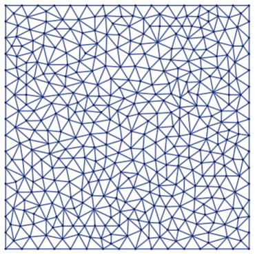
What will happen for a graph that is less regular than a grid? Here is a graph made by random triangulation of a 2D region:

And once again, the number of points reached at graph distance r grows like r²:

In ordinary d-dimensional continuous Euclidean space, the volume of a ball is exactly

And we should expect that if in some sense our graphs limit to d-dimensional space, then in correspondence with this, V_r should always show r^d growth.

There are, however, many subtle issues. The first—immediately evident in practice—is that if our graph is finite (like the grids above) then there are edge effects that prevent r^d growth in V_r when the radius of the ball becomes comparable to the radius of the graph. The pictures below show what happens for a grid with side length 11, compared to an infinite grid, and the r^d term on its own:

Table[With[{u = First[Values[ ResourceFunction["GraphNeighborhoodVolumes"][ GridGraph[Table[11, d]], GraphCenter[GridGraph[Table[11, d]]]]]]}, ListLinePlot[ Reverse@{Transpose[{Range[Length[u]] - 1, u}], Table[Evaluate[{r, FullSimplify@ FunctionExpand[ Binomial[r, d] Hypergeometric2F1[-d, 1 + r, 1 - d + r, -1]]}], {r, 0, Length[u] - 1}], Table[{r, 2^d/d! r^d}, {r, 0, Length[u - 1]}]}, Mesh -> All, Frame -> True, PlotRange -> {0, Max[u] + 1}, PlotStyle -> ResourceFunction["WolframPhysicsProjectStyleData"][ "GenericLinePlot", "PlotStyles"], If[d == 3, PlotLegends -> (Text[ Style[#, Directive[FontSize -> .85 Inherited, FontFamily -> "Source Serif Pro", GrayLevel[0.25]]]] & /@ {Style[Superscript["r", "d"], Italic], "infinite grid", "finite grid" }), PlotLegends -> None], Epilog -> Text[Style[Row[{Style["d", Italic], StringTemplate[" = ``"][d]}], Directive[FontSize -> 13, FontFamily -> "Source Serif Pro", GrayLevel[0.2]]], Scaled[{0, 1}], {-1.5, 1.3}]]], {d, 1, 3}]

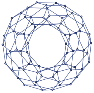
One might imagine that edge effects would be avoided if one had a toroidal grid graph such as:

Graph[ResourceFunction["TorusGraph"][{11, 7}], VertexStyle -> ResourceFunction["WolframPhysicsProjectStyleData"]["SpatialGraph", "VertexStyle"], EdgeStyle -> ResourceFunction["WolframPhysicsProjectStyleData"]["SpatialGraph", "EdgeLineStyle"]]

But actually the results for V_r(X) for any point on a toroidal graph are exactly the same as those for the center point in an ordinary grid; it is just that now finite-size effects come from paths in the graph that wrap around the torus.

Still, so long as r is small compared to the radius of the graph—but large enough that we can see overall r^d growth—we can potentially deduce an effective dimension from measurements of V_r.

In practice, a convenient way to assess the form of V_r, and to make estimates of dimension, is to compute log differences as a function of r:

Here are results for the center points of grid graphs (or for any point in the analogous toroidal graphs):

griddim[d_, s_] := ResourceFunction["LogDifferences"][ N[First[Values[ ResourceFunction["GraphNeighborhoodVolumes"][ GridGraph[Table[s, d]], GraphCenter[GridGraph[Table[s, d]]]]]]]]; GraphicsRow[{ListLinePlot[{griddim[1, 51], Table[{r, 1}, {r, 26}]}, PlotStyle -> {ResourceFunction["WolframPhysicsProjectStyleData"][ "GenericLinePlot", "PlotStyles"], Dotted}, PlotRange -> {0, 1.5}, Frame -> True], ListLinePlot[{griddim[2, 51], Table[{r, 2}, {r, 51}]}, PlotStyle -> {ResourceFunction["WolframPhysicsProjectStyleData"][ "GenericLinePlot", "PlotStyles"], Dotted}, Frame -> True], ListLinePlot[{griddim[3, 21], Table[{r, 3}, {r, 30}]}, PlotStyle -> {ResourceFunction["WolframPhysicsProjectStyleData"][ "GenericLinePlot", "PlotStyles"], Dotted}, Frame -> True]}, ImageSize -> Large]

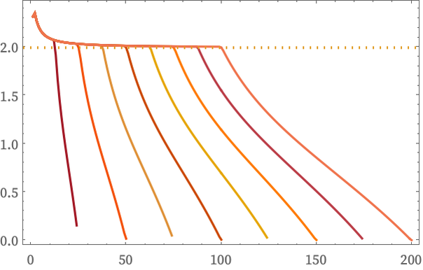
The results are far from perfect. For small r one is sensitive to the detailed structure of the grid, and for large r to the finite overall size of the graph. But, for example, for a 2D grid graph, as the size of the graph is progressively increased, we see that there is an expanding region of values of r at which our estimate of dimension is accurate:

griddim[d_, s_] := ResourceFunction["LogDifferences"][ N[First[Values[ ResourceFunction["GraphNeighborhoodVolumes"][ GridGraph[Table[s, d]], GraphCenter[ GridGraph[ Table[s, d]]]]]]]];(* griddata=Table[griddim[2,s],{s,25,200,25}] *) griddata = {{2.321928094887362, 2.356581185211473, 2.273087307226175, 2.216941690327061, 2.179126837524771, 2.152292761139919, 2.13235671871315, 2.1169935238862974`, 2.104804512968222, 2.0949039301137318`, 2.0867055636886356`, 2.0798067605722705`, 1.9252283343656778`, 1.6669708956150553`, 1.4593953099565267`, 1.2831913108682134`, 1.126843289342518, 0.9829140915168155, 0.8462402896565637, 0.7129739503358662, 0.5800317763245048, 0.4447517996502539, 0.30465844614280185`, 0.1572820700795648}, CompressedData[" 1:eJwBnQFi/iFib1JlAQAAADIAAABxo3kJT5MCQEzRhjxH2gJAu+nrZUgvAkDf v8jsS7wBQNMJKA3abgFAohtkROU3AUAWOxIKEQ8BQMl790ya7wBAr1+dv6PW AECDzeD9XMIAQDhkw6+SsQBAxkIVunGjAEDCNZV7ZJcAQC72eAX+jABAwkkk Me2DAECLRCpS9HsAQMD9EbbjdABACiTl5pVuAECn4gsR7WgAQMJ2OirRYwBA +JZCmy5fAECARHNE9VoAQOTpx8EXVwBAYsbO3IpTAEA1UdsR3///P366cNY7 Ov4/+NitExoZ/D+YLtxkADf6PzbEnETMhfg/5pmqLfz69j8xQ8RqkY71P6pw 7/pUOvQ/K1Ron1n58j8JzxzgpMfxP9b+fZLxofA/9yUI9gYL7z/r6O1IDeDs P34LzsHtvuo/T+uRIxqk6D/BNzwoYYzmP/NSe1bXdOQ/qDVzMcRa4j9X0FSR kjvgP/mvKIKGKdw/1+wDZsLH1z8m/UuF7UzTP6mig0sOaM0/2atLnMrvwz9D DKL3gky0PxYhSvAxsJQ/sRrBEA== "], CompressedData[" 1:eJwBXQKi/SFib1JlAQAAAEoAAABxo3kJT5MCQEzRhjxH2gJAu+nrZUgvAkDf v8jsS7wBQNMJKA3abgFAohtkROU3AUAWOxIKEQ8BQMl790ya7wBAr1+dv6PW AECDzeD9XMIAQDhkw6+SsQBAxkIVunGjAEDCNZV7ZJcAQC72eAX+jABAwkkk Me2DAECLRCpS9HsAQMD9EbbjdABACiTl5pVuAECn4gsR7WgAQMJ2OirRYwBA +JZCmy5fAECARHNE9VoAQOTpx8EXVwBAYsbO3IpTAECots8fRVAAQHCkeIE+ TQBAUoDaInBKAEA4HT0b1EcAQLYfhU5lRQBA1prBSx9DAEBqRhMy/kAAQNpz kJr+PgBAV98bhh09AEAm72FOWDsAQIfRXZmsOQBAw5LqThg4AEAFnv6PmTYA QCG0Zl59lf8/0ANKZo0C/j83BOVuj5P8PygMuA6OQvs/EhuQkcEK+j8wDiT4 R+j4PwR3XZfw1/c/qKfpXRXX9j99npfEfeP1P5iES7RI+/Q/Yn2bgdsc9D8T alas1EbzP71ZrXEBePI/J4E9glWv8T+g2chb5OvwP9QDdefbLPA/nwVNKgDj 7j+x06J7TnLtP8MvkUZuBuw/iFgA20Se6j94B40YzTjpPyC7mNMT1ec/HlXJ vDRy5j8OJASyVw/lP8s+vmSuq+M/y3o2RXJG4j95ARSl4t7gP4kQTgyG6N4/ RDiaF7ML3D+p9LEN2yXZPymM2CmMNdY/b+j7mVE50z9DT7/msC/QP6Eu8r9O Lso/jGA5B0/cwz9c2g9VWcy6P7CqMOREIqs/m5kI4w== "], CompressedData[" 1:eJwBLQPS/CFib1JlAQAAAGQAAABxo3kJT5MCQEzRhjxH2gJAu+nrZUgvAkDf v8jsS7wBQNMJKA3abgFAohtkROU3AUAWOxIKEQ8BQMl790ya7wBAr1+dv6PW AECDzeD9XMIAQDhkw6+SsQBAxkIVunGjAEDCNZV7ZJcAQC72eAX+jABAwkkk Me2DAECLRCpS9HsAQMD9EbbjdABACiTl5pVuAECn4gsR7WgAQMJ2OirRYwBA +JZCmy5fAECARHNE9VoAQOTpx8EXVwBAYsbO3IpTAECots8fRVAAQHCkeIE+ TQBAUoDaInBKAEA4HT0b1EcAQLYfhU5lRQBA1prBSx9DAEBqRhMy/kAAQNpz kJr+PgBAV98bhh09AEAm72FOWDsAQIfRXZmsOQBAw5LqThg4AEAFnv6PmTYA QDlSRK8uNQBAxvDRKtYzAEC2Wc+mjjIAQHKM4ehWMQBAxWg71C0wAEADKzlm Ei8AQPzPcLMDLgBAs30l5QAtAEDR8g43CSwAQK3BaPUbKwBAUuI+ezgqAEA8 /O4wXikAQEOAnNj7//8/jYPQwj8U/z/sBhiLNev9P6kchaw81vw/BSgCYcXS +z8GVznypN76P/5Pwb4C+Pk/P27WW0kd+T8ug7DSGk34P44XyD1Hhvc/jQ5O O8XH9j8ruiHNqxD2P2r38lctYPU/gkjYhZO19D8xNWbeOxD0P9/JofCUb/M/ FzPt8hvT8j/LRfjCWjryPxWjRzTmpPE/NjFon1wS8T+SqZ+mZILwPxFXHk5Y 6e8/19rbnc7R7j+rUrGln73tP4nEinpIrOw/i40MqE6d6z80DfEgP5DqPwJW Fk+thOk/zyB/PjJ66D8TeEjfa3DnPw7GM1v8ZuY/KNTke4ld5T8xCV8fvFPk P8vKpLg/SeM/r26l2sE94j8WyeLL8TDhP5jvaSGAIuA/iubIvzwk3j++jFND /f7bP8gkrIGm1Nk/Gf8BCZ2k1z+66YegRG7VPz5mmar/MNM/UYaJiC7s0D8u 9379XT7NP5joli+3ksg//+lRChbUwz+k9IPxPQK+P/7T7zzYMLQ/xoVW7S9i pD8RFUt8UJWEP98Kbtc= "], CompressedData[" 1:eJwNj3lQ1AUcxb8LkYGBcioRQyD3fYSwLPD9BiuHEjaECsohcgxRIwtYg62Q hYFyJSgZq5QEo3To6qyRI8myroAWSDsc4qIhlwHLfSyrLFu/P9585s28efOe 9ZHsmHQWAJxglNNwXHfvOS2KkhUHhsu1qGVKkR7hoUXD4gcze/5gUa+uo778 KIt+tEjjTvixyIxjpGe4hUUP+WtRgnkgYXKduGEAqKj7+UbCPSD/NKmw+iZQ R4jpnZwGoHu+Nfy0C0DuynwdTTnjI229ZouAyrjOMSt8oLYNw+axY0B6thMv ao4CXR3dbDibyeQ+C3CWpQKpvg256J4MdJKbx109CDQ+1SnZdgDoSMejp6Uf AjU191jt+gCI15j/ZfD7QDEn5Ta83cwOyyCLvnCgZquvo9N3AQ0IJHusQoGy woy9NQQkzzsr0AQDHRi2KLYMArKfT4mO4wCVyBJrf2UDSauno7f7A+l8r/mm dicQO4YrdPdlfi3InAd8mN74niuV3kC55SOT+72A2jM5fW6eQNou7AwjDyB1 D0+k7Q4kKrCbADcg2ZKBn64r0DVJ5qqFC7NzNJjv7wwUqJ7zTHIC+tzhcWm5 I/Nz0OUNqQPQBcW8F4uhlaeeIMweKOPhMXm1HZDH1qLzE7ZACQEcXjDDxliJ Rd0OIKdi2W4Ww5ju8OYsG6C5H0QWT6yBlt2VgVEMfeanhqXvAD0beWydL/4P mwPr6006NPjTraA8jXwD2WULXkK1Gi8dj8/rdVKjzSfChpCUdfxqzDxNVf8K Iz+2e2uL4iUees8lt4XzEmdPn2+MOKfC6yafxpkurqGiSuv1qtg1DF6vkrDv KrFTUpQgcFai6Avf7ohLq5guX5KNG66i/tMd7WZlK9h+Xyqo3LSC4l8EoF2y jBWm8oueusvoU/xz8pOKJSzhr6mkJkuY35Ua1VK3iIe/+1u70nERQ8MjnQx+ W0CWb2H31tAFtHxVwBtqnMebiSGhmvY55OqkToRMzWLb1WzzDINZjF/huTr6 zqDZoLI2KlGB+9dXbtcWT2NXWzxv8MYUjuvzlnqHJnHhBKcwftMkWjtss/f3 +Rfj7NYElPwCB3Jb17llE3hG7dq0/fdxvLtTaXZ2dAw/aq27flJ/DGfEkstt fqM4nlPUaZ8ygknGnadKzzxHNDcOK0kZRlaFTXbstWf4j+j0ZjflECY1jXZI OHIM5N/hSAsGcaaqv3WkZQCbPNJculf7MJF9X/iuSy/OiMoFHYdkaKny2XvY oAcfDF2pDTj4F0qH/3wzR9CJG4X7uPseSbFLoXLImhZjr32r9623b2NJRESN kfcN9O7vf00v5jL+DymQweQ= "], CompressedData[" 1:eJwNz3tUzAkUB/A7PdgKKVFrTKkwKaZGpJpp7l2KqI0mhGOrTZNYjyxnNzvs 9rDtOZkVJak8drfHKo8wxFa7qakhtskwZ2K2FWlKekxvWT3298c9n3PPueee 79cx+oBYwgKAs8wczD9itiHTiILVqcK1OiOq6OySBLobUUvVw+6gShY9M3OZ rtvPot/YMf76lSyaI7A2t7JkUb30fXCuAag08kJVvhYopeHV+I4aIO8YRWnG TSDlqtnlB/OBalZkSWOygXgjCaYTMmZft4DfkwJ0wt9VPCQFuj9uVfbmMJD5 An171n6g31strHrimLtvfF3VO4FGz67K40UCJfof8h/eDtTW+aDaNhwoWqlq TgsDulzW6BCwESi+ICFJ9DmQOFHnFL+eycHxY2vWApU5/BgiCQDS5lYHOawG 2rNm1rIJAtIdOpU7IQIKb2GncvyAFhm+DNkqAPpJ/UXOVR8gRca7EDtvINOL E+k5XkA+Yv9S3gqmV5/aVevJ/N3WWHRyGdDXstdvt/CB6uIEmqUeQMZuPrHW 7kBjjfFyYx6Q/NhCPSwFUg/MWGm2BOhaddww243J2SqSersCCcd6PSIWA33H bUqTuTA9n7t9ouACZXcZ+CxGBw/z3DWLgGLrD+syFgK5z0w5o18AtMNXEC9i LNhUzb7gDLQ4Vb2exShuWFu2xwmo95Kc/cIRaJA3Igxm9DR0tijmA1GOtQoZ XRM3aaocgDYW3qpZzWhTbL33sT0QZ/6Uoi2MTvJzgXoOUOMhJ963jPPQ3nMa 4/l9xl4F84DWvHCyRUaf86n3mtlAhYma8aOM5rndionJSXy8LoAtj5pE6Wiy IPrMBA7x7kbWq8dRLyscM7MbxzTJMCsidgxtT79Ls6n8iEr7Upt0u48YVS1w Qul/eDz5tm/Bmw94cPffy9aHfkDVtpu3HyhGsW/O5rFK31GsrK2qenrnPZ7u zhT+sfw93jOdJ+HeHUFjvruLTjiCO51NnmTWDWOh8MphdugwXqo78IOwZQhF 4Sqh8sAQhoSYSU8YDWHurRue0dmDKLt4U+TMG8Q9JmXTS5QD2Cd/tF8TNYAB 8ZLNyWP9OD1xSnFWTj++rKu3G1jZj7NPhQ0eberDe7vPGXES+jDa0fKr8k/7 sKJdyz6WYEANa04zt6oXX7Zn8IKn9mKvZsBSsbEH85zTvXfldWPL1OIRm44u VF27blHi2YWisM9kpknvkC+W10xt7MRfMv6alcHpxIgIH33q3rd4xeVsan1F B6obgC2y6MBYN8Px+u3tmFw+KQ4t0WOMzuR6xYc2fM63DzQEtmHjDUXws+w3 2LSkJHRDeyuqLXYHBi1vxTF1Q3xp0msUtDwIilG9wrcnmk+K575Cxz+dPZSP XuJkflLteMS/yApKHuT0/4OLVfdbRxN16OXHL42a8QKNbYfCuTlNmG6aUGzv qMWniVoXuyIN1srCJtu4z/DSrl795iI1Rpv2zBQ4PsFI61+9Hno04GUrvza0 fYQztmi/PzKsxJ9NFpZYPlZg4RlbXl72fYxTT8uS3CnHY5kXZ2m5t3F0X1Hg VosrWNux9yrbOw+3pc4V9kmk+D/TpRP5 "], CompressedData[" 1:eJwNz3k01XkYBvAvpk5EY01ZugjZurZjl/cdS3Y5mDRlOKOrjJG91dpYmkFF QpSasbZzmYwaEk5JC92SQrZ7Xdmvfe1e8/vjPZ/znvOe9zyPamC4V5AQIeQh NZElZ0UP5AijGyvN2rFHGP8bmwhy0hfGgcaXk671QvhBVEuiJ0wIixUZ9lwz IdxuJS0m9b0QtsUuuxXyCFYGFDWWdBFMfjvI92smaM5oqbzCJPjCVu5JZAnB ZpPcWEY+QfrSmU2CTGp3VjecSiaYYa/jtRBL8BlfqpYTQ1BMnTuSG0awgr1V aiqYujtlqcM6SnAlz/Y6PYBgkn20/eJhgsNjrU3yvgQDX7R/SfcmeLu2g+bg STCi9Mx5G3eCXkk9ahEuVA7lfYqdjgRraakeQQ4EuwqbXGl2BEP2yxgJkGBP dFahwIag74BimvI+gpq8XzwOWRG8wPq54L4FwZYr4x47zAluuim4XGBK0MLL vpJuQvWaYel0GVN/f+oov2REMCpzaPSgIcHnwVadew0IiuhaHJPWJ/itI6JG hE6wJl6DS/YSZM1tMxPVI/igKXhRUZfKybaJNdchaP1t2sBfm+C5PZ/SM7Wo np91t7TsIZg/wTMUoqQZiBXu1yR4rC2m54oGQX3J5KtcdYJ+llYRNpSlPk2K RbsJaqexXIQovd461oaoEZy+VaPYrUpwnr5k7UZpzBsbaFEhiAXS7UCpk+TT 2Ugj6FlW3WxHKXtHOvT1LoLKKpvLD1Kq1Vxz4ioT7IhWo5+mVIJdxuKUN06I mJYqEdzfrSYPlBY30uq+KBIsS+rkx1G21Rq9oVFKPqOLPVcg6IDlt0IpZbOZ J7dT5ghnnWreSbA/MfdiBOVq6c4KFcr4heNV73dQvZ2Z+WmUIShwtaaM/0ut YV6eYFw2s/c+pffTuWvHKTNk7fY8Ym3AlqzKc/LKG5DMbM1SiBDA7M3JXvVX fDgpY/n8ng4fjpzoGjTM/gYx6a8CHfjrMM4Qf5UQtg7mJj88Thxeg1/HTZdm /deg3dEpPa1vFfipnwQLAavA8epirnFX4JDVis3h8BUYcnm01rO+DLGsmjin jGWwkLxoFqW8DAsT+kq61UvwKZrh6Oy8BDVMnboy9iJsy/0ioZSwCJK9qu7p iotwZ4B7992TBfDBQj/WkQUIitQ5ESGYhwEr+byc4nngnLVTUnOahwujolXf 8eYg5g16auTPwTOfXv1wnIPrO9lF7eOz4N2QwjPImwUbfYnQFNtZoF9Psazj zUCJWL9nfdEMuC8nMc67zUCGo1rd7DIPZBTupWgf4sHtdYeYy4+nYVaPMSKq NA0JQbmQlDgFW8MCu3o4k3B68x9Dws6TIJ4cdZz9cAJmzProDLkJ8L8bWxUd Nw7NxbmifM4YzG5K4k26jkHRxECJwT+jcLe5bOyR0igwZJhrIalfobBKIsFm egSiyxsSaL4j4K0ncpTfyIU7ybThVi0uXObGbQ7PHgavFAtpzioHfnsilikb yIGR25H0hTY2yN8040QZsuHPir0N568NgXO/5pzUxiDoDml9lA0aBFl2/t/L VwdgOiyjJcK/H5QeGO8+o9kHtIAu9sxkL0z8+0H7KbMH0geqFVpiumFD5GAb 2+Qz2NI9DcliF/g99tITMD9CRsLD4MbQTvj4vi9AU+MDaFyScZfrZcHQ0dbd YZfeQZ5CuLhGQju4Ztedbu1+DSEJKQdS9dtgTe5qPC3xBeRPpaz/+LIFqsuY T7+KNYHH7wGOGhfroWCtvlpzqRbKB8fzXDyZoJqjYiRmWgEvi6PXlX3z4X8d qXKY "], CompressedData[" 1:eJwNz3s0FHgbB/Af6S2D3IoYmoxUaGdCWrc8zxvdEIVd7W6tU6u0NsVSWZeT jm3qSK/FKBQpU5a0uezSnTHHLSTSYCq3Go3LoDGyCvP+/njO5zznPOc536/F oRP+h9UIIY10Igt+0/TLUEefdp7bDok6PhoePbyTq4591Y1j3o/V8KXmeh3J cTW8yQzxlH6thkauBgx9XTVsipvxyZkgeC84t7pATDCptX9+fy1BpxDRvfQy gvVbVzyMLCBY65gZF3KFIOdTzOKFFLrvWmMnTyJ40dPGXxlHsGZev/JdNEHG GulQ5nGChYNa+vKj9O6Ui037TwT/vbz1KieYYKJnlOf09wTfDzcIjYMIHqp/ /iY5gOCflW2sbXsIRghizrrvJuifKGFHeNEc5luYnTsIVrLO+R7eRlCcI/Rm eRAM225ov4AEJVF/5Cy4EwzqY/LMtxBcO3HQd58rwfPtB7JLnAmK0kd8VzoR XJy3kJq9maCzv+c9jiPtNdluI3agf79ru/0/e4K/pgzIvrUjWHfUtfOrjQQX 2TofMeASnGuLqFjEIViRYCUlXxFsVyz7WnMDwbvCo9NMW5pz0D3OyYag29z4 xh+tCcau60pOWU97dtsuFa0jeGV0wk6NytrIyNm+luCRpmhJuhVBrl4SX7qG 4H4X1wh3qiBQyMy1JGjNa/dSo/q37qgMYxMcv17B7LEgOMX55OZDdZgY7hOt JojZBs+BapMY2FnNIrjnVnmtB3V5kcGx5lUEzVf/5/a3VHZF1k6pOcG2KDbn NNUMVjloU6+FL9osMCO4vYdtDFTna7z7b5gEbyV2zsdTmyrtW1hUvRoOo86U 4Da8ff0YdXla2Ukjaob6H6dqTQj2nsm8FEGdFZgUrqYmKENLO1bS3rvKrvCo Ybjg7UZNyGc/mTImGJ9W9rqEGvBUkRVKfWTYPWRJnd+qrBowIrh7JFKVT71s r1V2kFq1Tl1oSbUNNlnzYQXB3zddartDTQjTeRBJvelQJXai1p/TZalReyfn LzxbTjAkpUErk1qiiIhVqVRQduofbsV5FZCgnX4zowtQoCxXU3yzADwGXHSv m4cmryOtic7z4Gs1eCCkfA5ed2U9vMqdgyXxey73lX6Bq0eqXMYdv4DuFslc 8tPPUMVIEyZ4fQYZtyU1vWcW3hbOcLJ/mYWmYnlbCJkFqzjr6uYr/0KElgmr 0I6ayS/qaJ2Bp46C0xuOzcCrpu7nfO0ZsC7jT8n/+gRb/KpUzIBPUHON80Rj dhosStR/T82fBu+7ccxbu6bhefCyPK5SCXcT64JN85WgyxsS792tBLl9Fk/0 ZQoeNASNHrgzBexNuj/r7Z+C8ysFLs06U+AZ/vrQmRoFCPIj81ZFK2BvglfQ 1fUKqLS/niV7+xHUlxhqfM74CIWxOQ0ir49Q3m/Bd1H/CF6pg/yAh5Pw+H1Q qEbUJNiq6gw9NkxCevNFbe2WCZDdzNK7gBNgzMKTsn/G4VTxCZbZhnHI9htL MSiQA/unmGePTOVQ6J8dtjRjDH5gT8YPa42B6fcmvD3nRsFtWjOGqxqB7sC+ 4pjfRsDWw0S8SjkMIrPNjBUnhkHfr6jYd0QG4+esjlYflgHcd3D9YeAD5FXo Bxsd+AClog4fafcQ5DEfVz4OHAK9BUlS2gspEE5r8z4fKYgdHnYsaXwPJ3bH LOZ7vIeLip5pxdN34ORtEWTq8g4MZfzPqr8H4b82ji3Z3EGIarzU9rZoAEw/ 3DCrtRyAs86Tb9xy+2FTQ8pOT6N+0NTJ3Z5r3ge9oebRAp1eSFs5UZ089wbg pKjLbeQ1xFvF/lIolsBiO8b6KmEPlHTFlu+70w0ZpvKbMRldIA0sPbMoVgy5 c8H3pT++giQfzRtaWzvBuH1v+EHLlxCaesP2pXoHWJp61fj0vwDl8gBh1Ok2 sAi9ZKZt0woOjY2Wzt3PYOzVMvmLs43Aj+9dWrS2HgQvZk9frheBd6fWjfCD Qsgv3paiMf4EfN+NTPkuewAaCpl1sOXf8KAl9M/S7/4CwZxUXhUogJ/D2dHr jvMhuVNSw7gQDf8H/ozGnw== "]}; ListLinePlot[griddata, Epilog -> {Directive[ColorData[97, 2], Thick, Dotted], InfiniteLine[{0, 2}, {1, 0}]}, Frame -> True, PlotStyle -> ResourceFunction["WolframPhysicsProjectStyleData"][ "GenericLinePlot", "PlotStyles"]]

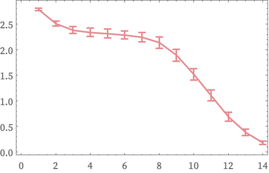
A notable feature of measuring dimension from the growth rate of V_r(X) is that the measurement is in some sense local: it starts from a particular position X. Of course, in looking at successively larger balls, V_r(X) will be sensitive to parts of the graph progressively further away from X. But still, the results can depend on the choice of X. And unless the graph is homogeneous (like our toroidal grids above), one will often want to average over at least a range of possible positions X. Here is an example of doing such averaging for a collection of starting points in the center of the random 2D graph above. The error bars indicate 1σ ranges in the distribution of values obtained from different points X.

rgraph = MeshConnectivityGraph[ DiscretizeRegion[Rectangle[], MaxCellMeasure -> .002], VertexSize -> Tiny, VertexStyle -> ResourceFunction["WolframPhysicsProjectStyleData"]["SpatialGraph", "VertexStyle"], EdgeStyle -> ResourceFunction["WolframPhysicsProjectStyleData"]["SpatialGraph", "EdgeLineStyle"]]; ListLinePlot[ ResourceFunction["LogDifferences"][ MeanAround /@ Transpose[ Values[ResourceFunction["GraphNeighborhoodVolumes"][rgraph, VertexList[NeighborhoodGraph[rgraph, GraphCenter[rgraph], 1]], Automatic]]]], Frame -> True, PlotStyle -> ResourceFunction["WolframPhysicsProjectStyleData"][ "GenericLinePlot", "PlotStyles"]]

So far we have looked at graphs that approximate standard integer-dimensional spaces. But what about fractal spaces [23]? Let us consider a Sierpiński graph, and look at the growth of a ball in the graph:

Module[{cg, sier = IndexGraph[MeshConnectivityGraph[SierpinskiMesh[6], 0], VertexStyle -> ResourceFunction["WolframPhysicsProjectStyleData"][ "SpatialGraph", "VertexStyle"], EdgeStyle -> ResourceFunction["WolframPhysicsProjectStyleData"][ "SpatialGraph", "EdgeLineStyle"]]}, cg = First[GraphCenter[sier]]; Table[Labeled[ HighlightGraph[sier, NeighborhoodGraph[sier, cg, r], ImageSize -> 140], Text[Style[Row[{Style["r", Italic], StringTemplate[" = ``"][r]}], Directive[GrayLevel[.25], FontSize -> .85 Inherited, FontFamily -> "Source Serif Pro" ]]]], {r, 5, 20, 5}]]

Estimating dimension from V_r(X) averaged over all points we get (for graphs made from 6 and 7 recursive subdivisions):

GraphicsRow[ Table[Module[{sier = IndexGraph[MeshConnectivityGraph[SierpinskiMesh[ss], 0]], w}, w = ResourceFunction["LogDifferences"][ MeanAround /@ Transpose[ Values[ResourceFunction["GraphNeighborhoodVolumes"][sier, All, Automatic]]]]; ListLinePlot[{w, Table[{r, Log[2, 3]}, {r, Length[w]}]}, PlotStyle -> {ResourceFunction["WolframPhysicsProjectStyleData"][ "GenericLinePlot", "PlotStyles"], Dotted}, Frame -> True]], {ss, 6, 7}], ImageSize -> Large]

The dotted line indicates the standard Hausdorff dimension log₂(3)≈1.58 for a Sierpiński triangle [23]. And what the pictures suggest is that the growth rate of V_r approximates this value. But to get the exact value we see that in addition to everything else, we will need average estimates of dimension over different values of r.

In the end, therefore, we have quite a collection of limits to take. First, we need the overall size of our graph to be large. Second, we need the range of values of r for measuring V_rto be small compared to the size of the graph. Third, we need these values to be large relative to individual nodes in the graph, and to be large enough that we can readily measure the leading order growth of V_r—and that this will be of the form r^d. In addition, if the graph is not homogeneous we need to be averaging over a region X that is large compared to the size of inhomogeneities in the graph, but small compared to the values of r we will use in estimating the growth of V_r. And finally, as we have just seen, we may need to average over different ranges of r in estimating overall dimension.

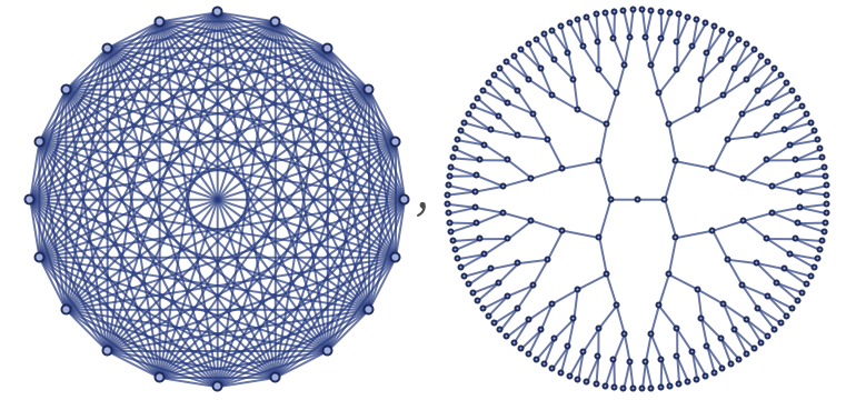
If we have something like a grid graph, all of this will work out fine. But there are certainly cases where we can immediately tell that it will not work. Consider, for example, first the case of a complete graph, and second of a tree:

{CompleteGraph[20, Sequence[ VertexStyle -> ResourceFunction["WolframPhysicsProjectStyleData"][ "SpatialGraph", "VertexStyle"], EdgeStyle -> ResourceFunction["WolframPhysicsProjectStyleData"][ "SpatialGraph", "EdgeLineStyle"]]], TreePlot[KaryTree[255], Center, Sequence[ VertexStyle -> ResourceFunction["WolframPhysicsProjectStyleData"][ "SpatialGraph", "VertexStyle"], EdgeStyle -> ResourceFunction["WolframPhysicsProjectStyleData"][ "SpatialGraph", "EdgeLineStyle"]]]}

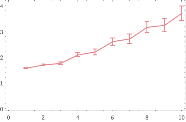
For a complete graph there is no way to have a range of r values “smaller than the radius of graph” from which to estimate a growth rate for V_r. For a tree, V_r grows exponentially rather than as a power of r, so our estimate of dimension Δ(r) will just continually increase with r:

ListLinePlot[ ResourceFunction["LogDifferences"][ MeanAround /@ Transpose[ Values[ResourceFunction["GraphNeighborhoodVolumes"][ KaryTree[2047], All, Automatic]]]], Frame -> True, PlotStyle -> ResourceFunction["WolframPhysicsProjectStyleData"][ "GenericLinePlot", "PlotStyles"]]

But notwithstanding these issues, we can try applying our approach to the objects generated by our models. As constructed, these objects correspond to directed graphs or hypergraphs. But for our current purposes, we will ignore directedness in determining distance, effectively taking all elements in a particular k-ary relation—regardless of their ordering—to be at unit distance from each other.

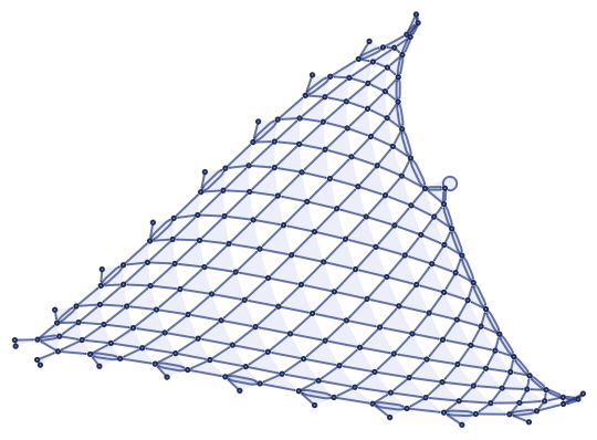
As a first example, consider the 2₃  3₃ rule we discussed above that “knits” a simple grid:

ResourceFunction[ "WolframModel"][{{1, 2, 2}, {3, 1, 4}} -> {{2, 5, 2}, {2, 3, 5}, {4, 5, 5}}, {{0, 0, 0}, {0, 0, 0}}, 200, "FinalStatePlot"]

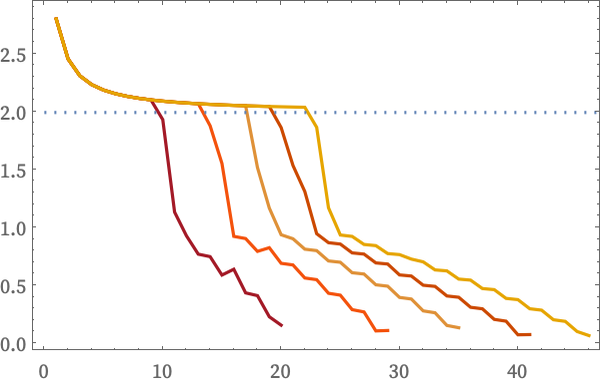
As we run the rule, the structure it produces gets larger, so it becomes easier to estimate the growth rate of V_r. The picture below shows Δ(r) (starting at the center point) computed after successively more steps. And we see that, as expected, the dimension estimate appears to converge to value 2:

CenteredDimensionEstimateList[g_Graph] := ResourceFunction["LogDifferences"][ N[First[Values[ ResourceFunction["GraphNeighborhoodVolumes"][g, GraphCenter[g]]]]]]; Show[ListLinePlot[ Table[CenteredDimensionEstimateList[ UndirectedGraph[ ResourceFunction["HypergraphToGraph"][ ResourceFunction[ "WolframModel"][{{1, 2, 2}, {3, 1, 4}} -> {{2, 5, 2}, {2, 3, 5}, {4, 5, 5}}, {{0, 0, 0}, {0, 0, 0}}, t, "FinalState"]]]], {t, 500, 2500, 500}], Frame -> True, PlotStyle -> ResourceFunction["WolframPhysicsProjectStyleData"][ "GenericLinePlot", "PlotStyles"]], Plot[2, {r, 0, 50}, PlotStyle -> Dotted]]

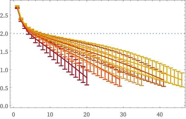
It is worth mentioning that if we did not compute V_r(X) by starting at the center point, but instead averaged over all points, we would get a less useful result, dominated by edge effects:

HypergraphDimensionEstimateList[hg_] := ResourceFunction["LogDifferences"][ MeanAround /@ Transpose[ Values[ResourceFunction["HypergraphNeighborhoodVolumes"][hg, All, Automatic]]]]; Show[ListLinePlot[ Table[HypergraphDimensionEstimateList[ ResourceFunction[ "WolframModel"][{{1, 2, 2}, {3, 1, 4}} -> {{2, 5, 2}, {2, 3, 5}, {4, 5, 5}}, {{0, 0, 0}, {0, 0, 0}}, t, "FinalState"]], {t, 500, 2500, 500}], Frame -> True, PlotStyle -> ResourceFunction["WolframPhysicsProjectStyleData"][ "GenericLinePlot", "PlotStyles"]], Plot[2, {r, 0, 50}, PlotStyle -> Dotted]]

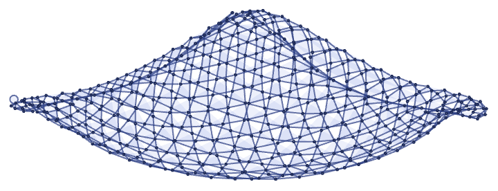
As a second example, consider the 2₃ 3₃ rule that slowly generates a somewhat complex kind of surface:

ResourceFunction[ "WolframModel"][{{1, 1, 2}, {1, 3, 4}} -> {{4, 4, 5}, {5, 4, 2}, {3, 2, 5}}, {{0, 0, 0}, {0, 0, 0}}, 500, "FinalStatePlot"]

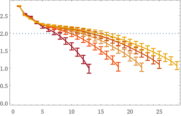
As we run this longer, we see what appears to be increasingly close approximation to dimension 2, reflecting the fact that even though we can best draw this object embedded in 3D space, its intrinsic surface is two-dimensional (though, as we will discuss later, it also shows the effects of curvature):

HypergraphDimensionEstimateList[hg_] := ResourceFunction["LogDifferences"][ MeanAround /@ Transpose[ Values[ResourceFunction["HypergraphNeighborhoodVolumes"][hg, All, Automatic]]]]; Show[ListLinePlot[ Table[HypergraphDimensionEstimateList[ ResourceFunction[ "WolframModel"][{{1, 1, 2}, {1, 3, 4}} -> {{4, 4, 5}, {5, 4, 2}, {3, 2, 5}}, {{0, 0, 0}, {0, 0, 0}}, t, "FinalState"]], {t, 500, 2500, 500}], Frame -> True, PlotStyle -> ResourceFunction["WolframPhysicsProjectStyleData"][ "GenericLinePlot", "PlotStyles"]], Plot[2, {r, 0, 50}, PlotStyle -> Dotted]]

The successive dimension estimates shown above are spaced by 500 steps in the evolution of the rule. As another example, consider the 2₃1₂  4₃4₂ rule, in which geometry emerges rapidly through a process of subdivision:

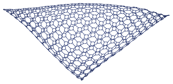
ResourceFunction[ "WolframModel"][{{1, 2, 3}, {4, 5, 6}, {1, 4}} -> {{2, 7, 8}, {3, 9, 10}, {5, 11, 12}, {6, 13, 14}, {13, 8}, {7, 10}, {9, 12}, {11, 14}}, {{0, 0}, {0, 0}, {0, 0}, {0, 0, 0}, {0, 0, 0}}, 9, "FinalStatePlot"]

These are dimension estimates for all of the first 10 steps in the evolution of this rule:

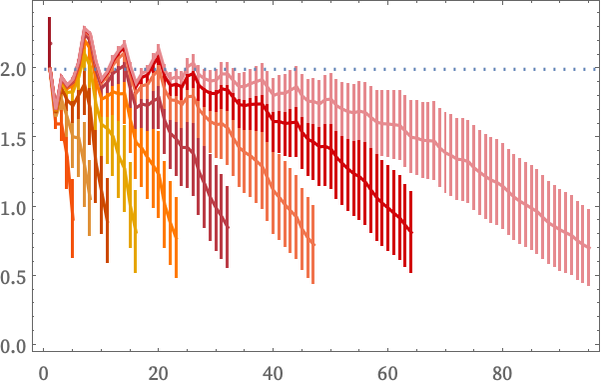
HypergraphDimensionEstimateList[hg_] := ResourceFunction["LogDifferences"][ MeanAround /@ Transpose[ Values[ResourceFunction["HypergraphNeighborhoodVolumes"][hg, All, Automatic]]]]; Show[ListLinePlot[ Table[HypergraphDimensionEstimateList[ ResourceFunction[ "WolframModel"][{{1, 2, 3}, {4, 5, 6}, {1, 4}} -> {{2, 7, 8}, {3, 9, 10}, {5, 11, 12}, {6, 13, 14}, {13, 8}, {7, 10}, {9, 12}, {11, 14}}, {{0, 0}, {0, 0}, {0, 0}, {0, 0, 0}, {0, 0, 0}}, t, "FinalState"]], {t, 1, 10}], Frame -> True, PlotStyle -> ResourceFunction["WolframPhysicsProjectStyleData"][ "GenericLinePlot", "PlotStyles"]], Plot[2, {r, 0, 100}, PlotStyle -> Dotted]]

We can also validate our approach by looking at rules that generate obviously nested structures. An example is the 2₂  4₂ rule that produces:

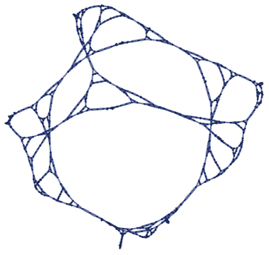
ResourceFunction[ "WolframModel"][{{1, 2}, {3, 2}} -> {{2, 4}, {2, 4}, {4, 1}, {3, 4}}, {{0, 0}, {0, 0}, {0, 0}}, 12, "FinalStatePlot"]

The results for each of the first 15 steps show good correspondence to dimension log₂(3)≈1.58:

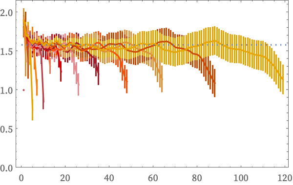
HypergraphDimensionEstimateList[hg_] := ResourceFunction["LogDifferences"][ MeanAround /@ Transpose[ Values[ResourceFunction["HypergraphNeighborhoodVolumes"][hg, All, Automatic]]]]; Show[ListLinePlot[ Table[HypergraphDimensionEstimateList[ ResourceFunction[ "WolframModel"][{{1, 2}, {3, 2}} -> {{2, 4}, {2, 4}, {4, 1}, {3, 4}}, {{0, 0}, {0, 0}, {0, 0}}, t, "FinalState"]], {t, 1, 15}], Frame -> True, PlotRange -> {0, Automatic}, PlotStyle -> ResourceFunction["WolframPhysicsProjectStyleData"][ "GenericLinePlot", "PlotStyles"]], Plot[Log[2, 3], {r, 0, 150}, PlotStyle -> Dotted]]

A Class of Models with the Potential to Represent Fundamental Physics

4.5 The Notion of Dimension