8.4 The Structure of Space

In our models, the structure of spacetime is defined by the structure of the evolving hypergraph. Causal foliations of the evolution can be used to define spacelike hypersurfaces. The instantaneous structure of space (on a particular spacelike hypersurface) corresponds to a particular state of the hypergraph.

A position in space is defined by a node in the hypergraph. A geometrical distance between positions can be defined as the number of hyperedges on the shortest path in the hypergraph between them. Although the underlying rules for hypergraph rewriting in our models depend on the ordering of elements in hyperedges, this is ignored in computing geometrical distance. (The geometrical distance discussed here is basically just a proxy for a true physical distance measured from dynamic information transmission between positions.) A shortest path on the hypergraph between two positions defines a geodesic between them, and can be considered to define a straight line.

The only information available to define the structure of space is the connectivity of the hypergraph; there is no predefined embedding or topological information. The continuum character of space assumed in traditional physics must emerge as a large-scale limit of the hypergraph (somewhat analogously to the way the continuum character of fluids emerges as a large-scale limit of discrete molecular dynamics (e.g. [1:p378][110]). Although our models follow definite rules, they can intrinsically generate effective randomness (much like the rule 30 cellular automaton, or the computation of the digits of π). This effective randomness makes large-scale behavior typically approximate statistical averages of small-scale dynamics.

In our models, space has no intrinsic dimension defined; its effective dimension must emerge from the large-scale structure of the hypergraph. Around every node at position X consider a geodesic ball consisting of all nodes that are a hypergraph distance not more than r away. Let V_r(X) be the total number of nodes in this ball. Then the hypergraph can be considered to approximate d-dimensional space if

for a suitable range of values of r. Here we encounter the first of many limits that must be taken. We want to consider the limit of a large hypergraph (say as generated by a large number of steps of evolution), and we want r to be large compared to 1, but small compared to the overall diameter of the hypergraph.

As a simple example, consider the hypergraph created by the rule

Starting from a minimal initial condition of two self-loops, the first few steps of evolution with our standard updating order are:

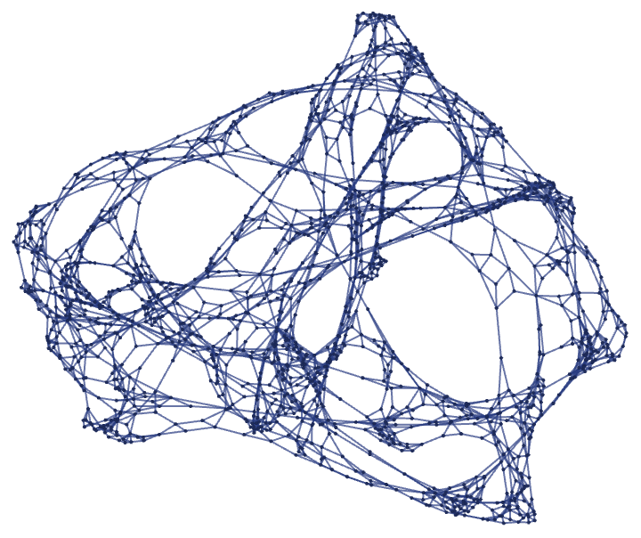
The hypergraph obtained after 12 steps has 1651 nodes and can be rendered as:

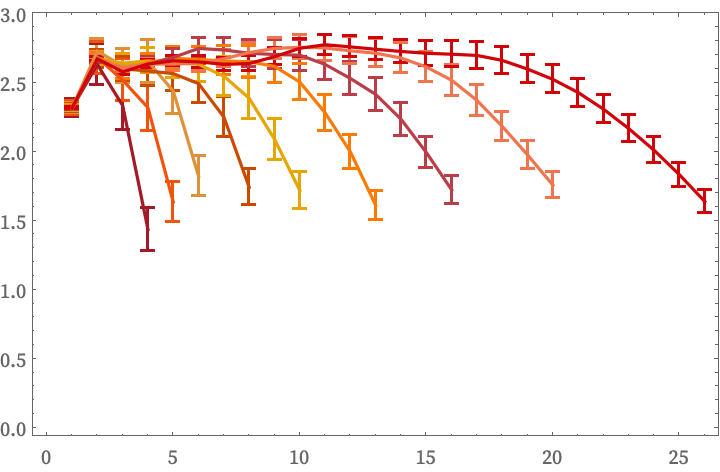
This plots the effective “dimension exponent” of r in V_r as a function of r, averaged over all nodes in the hypergraph, for a succession of steps in the evolution:

A constant limiting value d indicates approximation to a “flat” d-dimensional space. For integer d, this corresponds to ordinary d-dimensional Euclidean space, but in our models d often does not end up being integer valued, nor does it need to be constant at different positions, or through the course of evolution. It is also important to note that only some rules give V_r~ r^d; exponential or more complex behavior is common.

Even when to leading order V_r~ r^d, there are corrections. For small r (measured, say, relative to the diameter of the hypergraph) one can consider a power series expansion in r. By comparison to ordinary manifolds one can then write (e.g. [24][1:p1050])

where R can be identified as the (Ricci) scalar curvature [25][26] of the limiting space. The value of this curvature is again purely determined by the (limiting) structure of the hypergraph. (Note that particularly if one goes beyond a pure power series, there is the potential for subtle interplay between change in dimension and what one might attribute to curvature.)

It is also possible to identify other limiting features of the hypergraph. For example, consider a small stretch of geodesic (where by “small” we mean still large compared to individual connections in the hypergraph, but small compared to the scale on which statistical features of the hypergraph change). Now create a tube of radius r by including every node with distance up to r from any node on the geodesic. The growth rate of the number of nodes in this tube can then be approximated as [44]

where now R_ijδxⁱδx^j is the projection of the Ricci tensor along the direction of the geodesic. (The Ricci tensor measures the change in cross-sectional area for a bundle of geodesics, associated with their respective convergence and divergence for positive and negative curvature.)

In a suitable limit, the nodes in the hypergraph correspond to points in a space. A tangent bundle at each point can be defined in terms of the equivalence class of geodesics through that point, or in our case the equivalence class of sequences of hyperedges that pass through the corresponding node in the hypergraph.

One can set up what in the limit can be viewed as a rank-p tensor field on the hypergraph by associating values with p hyperedges at each node. When these values correspond to intrinsic features of the hypergraph (such as V_r), their limits give intrinsic properties of the space associated with the hypergraph. And for example the Riemann tensor can be seen as emerging from essentially measuring areas of “rectangles” defined by loops in the hypergraph, though in this case multiple limits need to be taken.