5.8 Causal Graphs for Particular Updating Sequences

The multiway causal graph that we have just constructed shows the causal relationships for all possible paths of evolution in a multiway system. But what if we just pick a single path of evolution? Instead of looking at the results for every possible updating order, let us pick a particular updating order.

For example, for the rule above we could pick “sequential updating”, in which at each step, first for AB  BAB and then for BA  A, we scan the string from left to right, doing the first replacement we can [1:3.6]. This leads to a specific single path of evolution for the system (now drawn across the page):

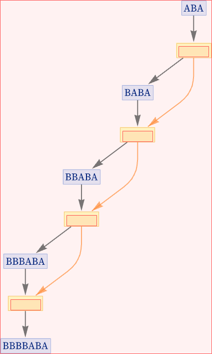
We can show the causal relationships between the events in this evolution:

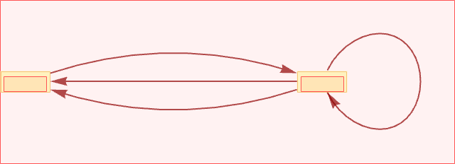
And we can generate a causal graph—which is very simple:

But now let us consider a different updating scheme, in which now as we scan the string, we try at each position both AB  BAB and BA  A, then do the first replacement we can. This procedure again leads to a specific single path of evolution, but it is a different one from before:

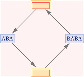
This particular path just involves an alternation between the states ABA and BABA, so the states graph is a cycle:

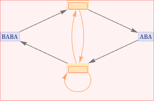
Including causal relationships here we get:

The resulting causal graph is then:

This causal graph is quite different from the one we got for the previous updating scheme. But both individual causal graphs necessarily occur in the whole multiway causal graph:

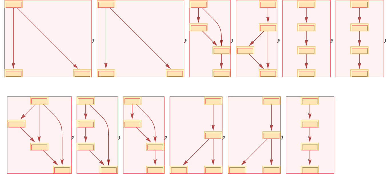
Given the multiway causal graph, we can explicitly find all possible individual causal graphs (not showing individual loop configurations separately):

And what this shows is that at least with the particular rule we are looking at, there are many different classes of evolution paths, that can lead to distinctly different individual causal graphs—and therefore causal histories.