Just as states that occur at successive steps in the evolution of our underlying systems can be thought of as associated with successive slices in a foliation of the causal graph, so also branchial graphs can be thought of as being associated with successive slices in a foliation of the multiway graph.
As we discussed above, different foliations of the causal graph define different relative orderings of updating events within our underlying system. But we can now think about this at a higher level and consider foliations of the multiway graph, that in effect define different relative orders of updating events on different branches of the multiway system. A foliation of the causal graph in effect defines how we should line up our notion of “time” for events in different parts of our underlying system; a foliation of the multiway graph now also defines how we should line up our notion of “time” for events on different branches of the multiway system.
For example, with the rule
starting from AA, we can define the following foliation of the multiway graph:
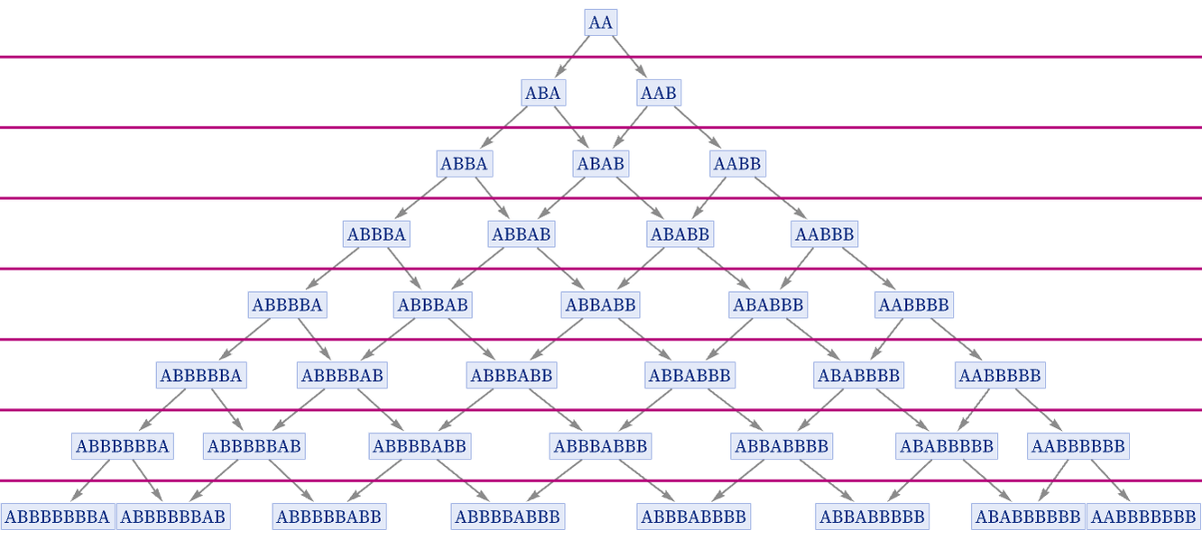
This yields the branchial graphs:
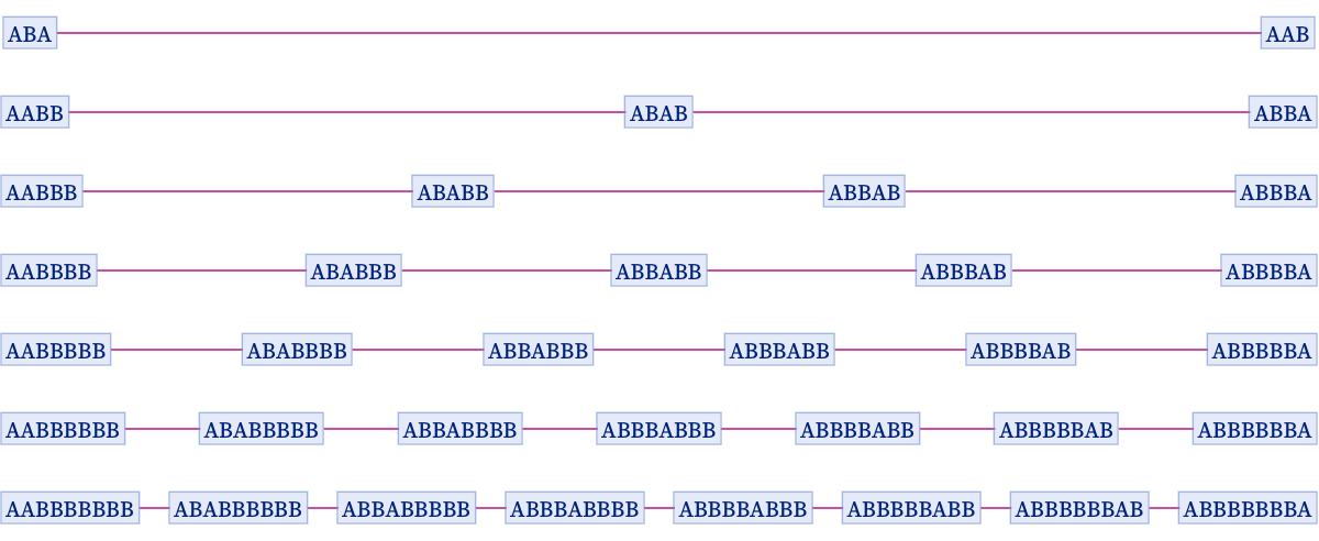
Just as the causal graph defines a partial order for events, so now the multiway graph defines a partial order for states. And so long as it is consistent with this partial order, we can pick any total order for the states. And we can parametrize some of these total orders as foliations.
For the particularly simple case shown here, an alternative foliation consistent with the partial order defined by the multiway system is:
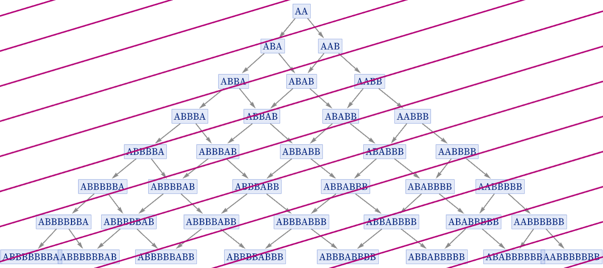
And if we use this foliation, we get a different sequence of branchial graphs, now no longer connected:
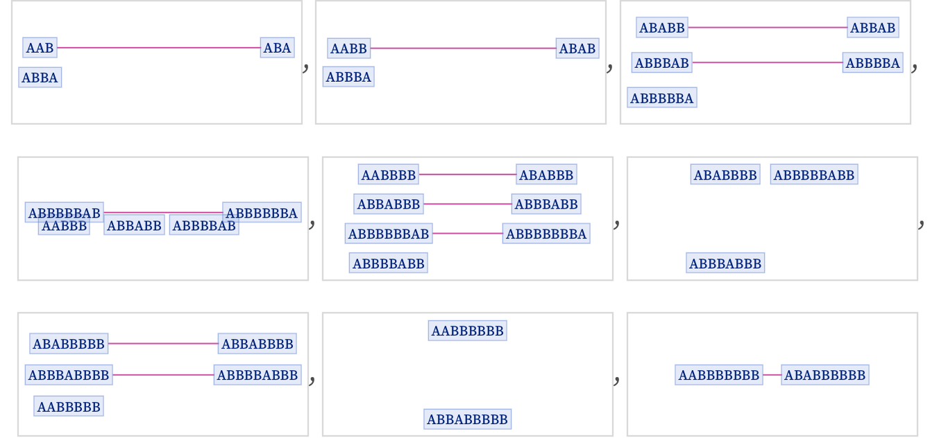
This example is particularly obvious in its analogy with the causal graphs we discussed above. But what makes this work is a special feature of the branchial graphs in this case: the fact that the states that appear in them can in effect be assigned simple 1D “coordinates”. In the original foliation with unslanted (“one event per slice”) slices, the “coordinate” is effectively just the position of the second A in the string. And with respect to the “space” defined by this “coordinate”, the branchial graphs can readily be laid out in one dimension, and we can readily set up “slanted” foliations, just like we did for causal graphs.
With the underlying systems we are discussing in this section being based on strings of elements, it is inevitable that there will be 1D coordinates that can be assigned to the events that occur in the causal graph. But nothing like this need be true of the branchial graph, and indeed most branchial graphs have a significantly more complex structure.
Consider the same rule as above, but now started from AAA. The multiway graph in this case—with a foliation indicated—is then:
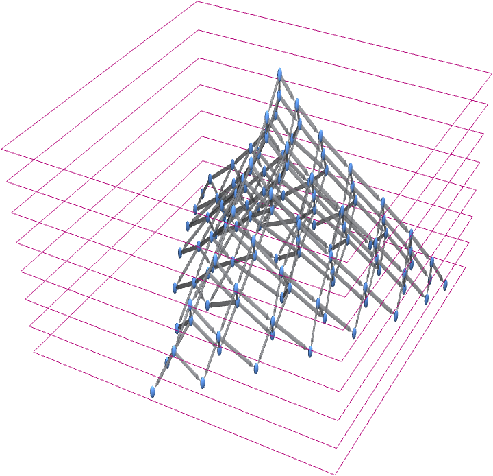
The branchial graphs now have a two-dimensional structure—with the positions of the second and third As in each string providing potential “coordinates”:
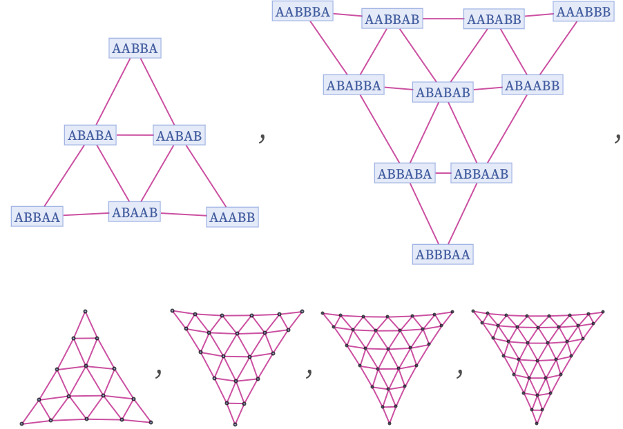
But consider now the rule
started from BABABABA. The multiway graph in this case is:
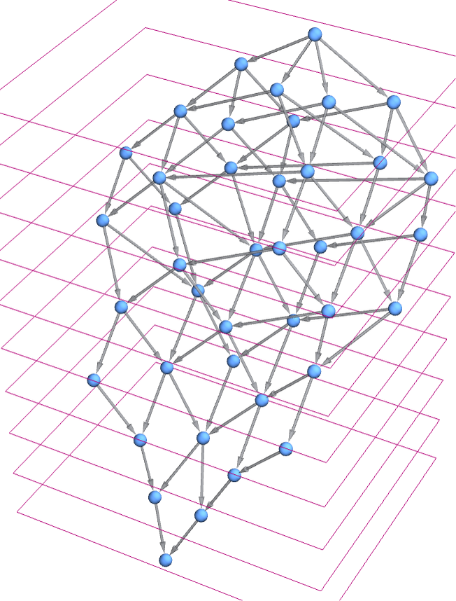
And the sequence of branchial graphs based on the foliation above is now:
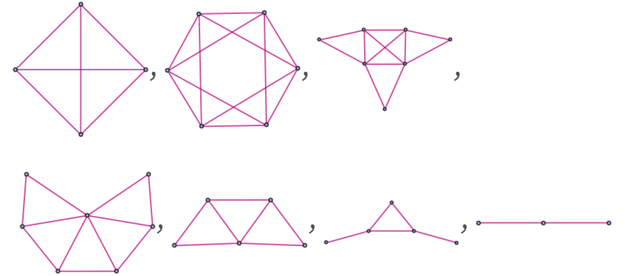
But here it is already much less clear how to assign “coordinates” in “branchial space”, or how to create a meaningful family of foliations of the multiway graph.
In thinking about multiway graphs and their foliations there is another complication that can arise for some rules. Consider two versions of the multiway graph for the rule:

In the first version, every distinct state is shown only once. But in the second case, the evolution is “partially unrolled” to show separately different instances of the same state, produced after different numbers of updating events. With a foliation whose slices correspond to the layers in the renderings above, the first version of the multiway system yields the branchial graphs:

The second version, however, yields different branchial graphs:

To some extent this difference is just like taking a different foliation. But there is more to it, because the second version of the multiway graph actually defines different ordering constraints than the first one. In the second version, there is a true partial ordering, defined by the directed edges in the multiway graph. But in the first version, there can be loops, and so no strict partial order is defined. (We will discuss this phenomenon more in 6.9.)
 download pdf
  ARXIV
ARXIV peer review