5.3 States Graphs

If there are multiple successors to a particular state in a substitution system one thing to do would be just to assume that each of these successors is a new, unique state. The result of this will always be to produce a tree of states, here shown for the rule {A  BBB, BB  A}:

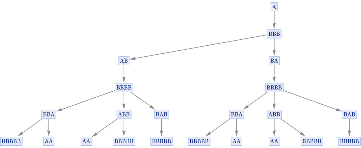
But in our construction of multiway systems, we assume that actually the states produced are not all unique, and instead that states at a given step consisting of the same string can be merged, thereby reducing the tree above to the directed graph:

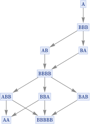
But if we are going to merge identical states, why do so only at a given step? Why not merge identical states whenever they occur in the evolution of the system? After all, given the setup, a particular state—wherever it occurs—will always evolve in the same way, so in some sense it is redundant to show it multiple times.

The particular rule {A  BBB, BB  A} that we have just used as an example has the special feature that it always “makes progress” and never repeats itself—with the result that a given string only ever appears once in its evolution. Most rules, however, do not have this property.

Consider for example the rule {AB  BAB, BA  A}. Starting from ABA, here is our normal “evolution graph”:

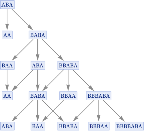
Notice that in this evolution even the original state ABA appears again, both at step 3 and at step 5—and each time it appears, it necessarily makes a complete repeat of the same evolution graph. To remove this redundancy, we can make a graph in which we effectively merge all instances of a given state, so that we show each state only once, connecting it to whatever states it evolves to under the rule:

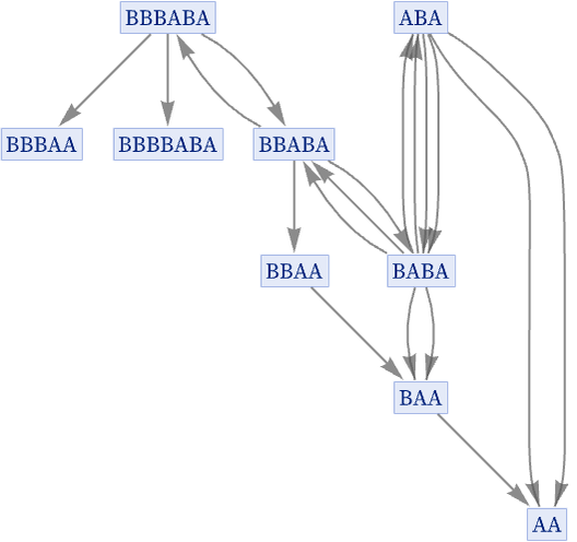
But in this graph there are, for example, two connections from ABA to BABA, because this transformation happens twice in the 4 steps of evolution that we are considering. But in a sense this multiplicity again always gives redundant information, so in what we will call our “states graph” [1:p209], we only ever keep one connection between any given pair of states, so that in this case we get:

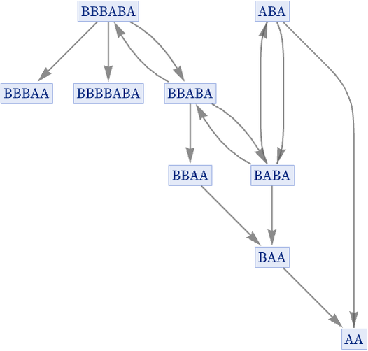
There is one further subtlety in the construction of a states graph. The graph only records which state can be transformed into which other: it does not record how many different replacements could be applied to achieve this. In the rule we just showed, it is never possible to have different replacements on a single string yield the same result.

Consider the rule {A  AA, A  B} starting with AA. There are, for example, two different ways that this rule can be applied to AA to get AAA:

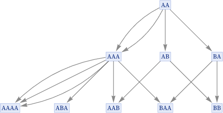
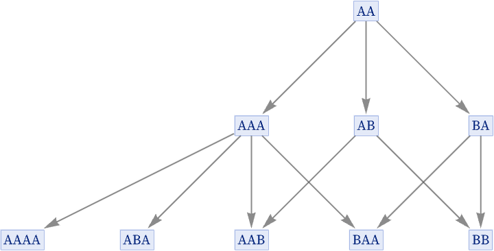
In our standard states graph, however, we show only that AA is transformed to AAA, and we do not record how many different possible replacements can achieve this:

The degree of compression achieved in going from evolution graphs to states graphs can be quite dramatic. For example, for the rule {BA  AB, AB  BA} the evolution graph is

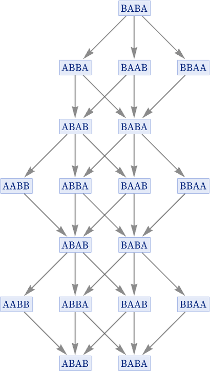
and the states graph is

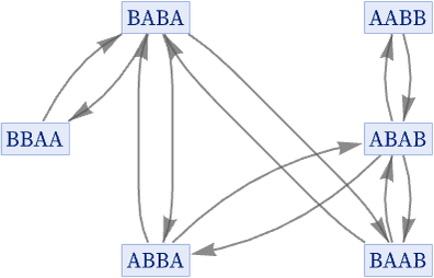
or in our standard rendering:

Note that causal invariance works the same in states graphs as it does in evolution graphs: if a rule is causal invariant, any two paths that diverge must eventually reconverge.