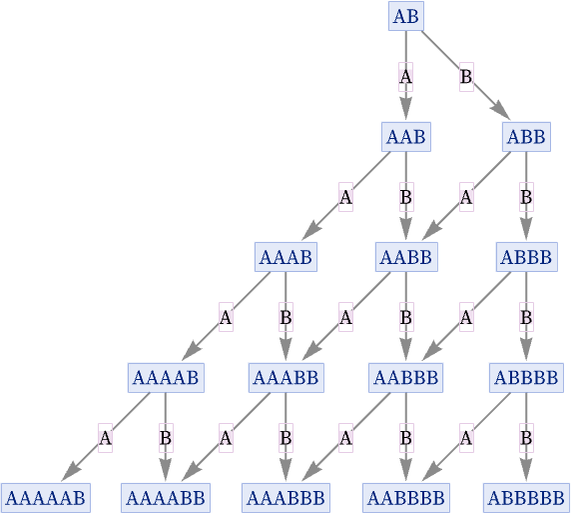
Causal invariance implies that regardless of the order in which updates are made, it is always possible to get to the same outcome. One way this can happen is if different updates can never interfere with each other. Consider the rule {A AA, B BB}. Every time one sees an A, it can be “doubled”, and similarly with a B. But these doublings can happen independently, in any order. Looking at an evolution graph for this rule we see that at each state there can be an “A replacement” applied, or a “B replacement”. There are two branches of evolution depending on which replacement is chosen, but one can always eventually reach the same outcome, regardless of which choice was made—and as a result the rule is causal invariant:
The replacements A AA and B BB trivially cannot interfere because their left-hand sides involve different elements. But a more general way to guarantee that interference cannot occur is for the left-hand sides of replacements not to be able to overlap with each other—or with themselves.
In general, the set of strings of As and Bs up to length 5 that do not overlap themselves are (up to A,B interchange and reversal): [1:p1033][59]
These can be formed into pairs in the following ways:
The first triples with no overlaps are of length 6. An example is {AAABB, ABAABB, ABABB}. And whenever there is a set of strings with no overlaps being used as the left-hand side of replacements, one is guaranteed to have a system that is totally causal invariant.
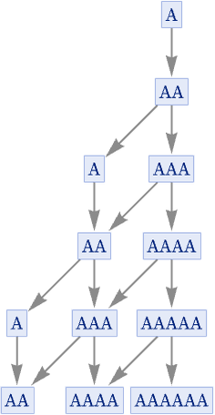
It is also perfectly possible for the right-hand sides of rules to be such that the system is totally causal invariant even though their left-hand sides overlap. An example is the simple rule {A AA, AA A}:
At every branch point in a multiway system, one can identify all pairs of strings that can be generated. We will call such pairs of strings branch pairs (they are often called “critical pairs” [60]). And the question of whether a system is causal invariant is then equivalent to the question of whether all branch pairs that can be generated will eventually resolve, in the sense that there is a common successor for both members of the pair [61][62][63][64].
Consider for example the rule {A AB, B A}:
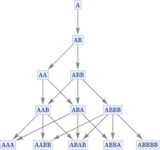
After two steps, a branch pair appears: {AA, ABB}. But after just one more step it resolves. However, two more branch pairs are generated: {AAB, ABA} and {ABA, ABBB}. But after another step, these also resolve. And in fact in this system all branch pairs that are ever generated resolve (actually always in just one step), and so the system is causal invariant.
In general, it can, however, take more than one step for a branch pair to resolve. The simplest case involving resolution after two steps involves the rule:
The state AB generates the branch pair {BB, AA}:
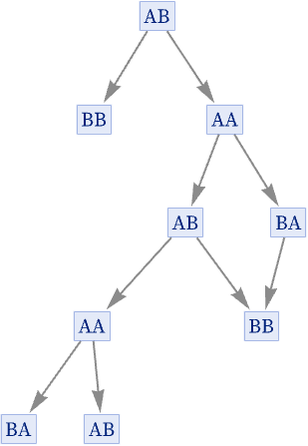
In the evolution graph, we do not see a resolution of this branch pair. But looking at the states graph, we see that the branch pair does indeed resolve in two steps, though with BB being a terminating state:
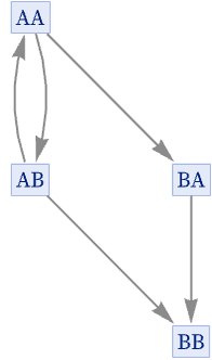
The same kind of thing can also happen without a terminating state. Consider for example
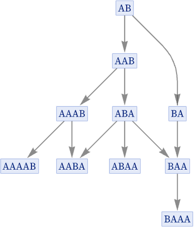
where the branch pair {AAB, BA} takes 2 steps to resolve.
In the rule
it takes 3 steps for the branch pair {AAAB, BA} to resolve:
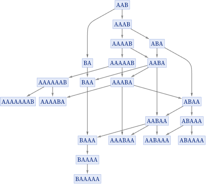
Things can get quite complicated even with simple rules. For example, in the rule
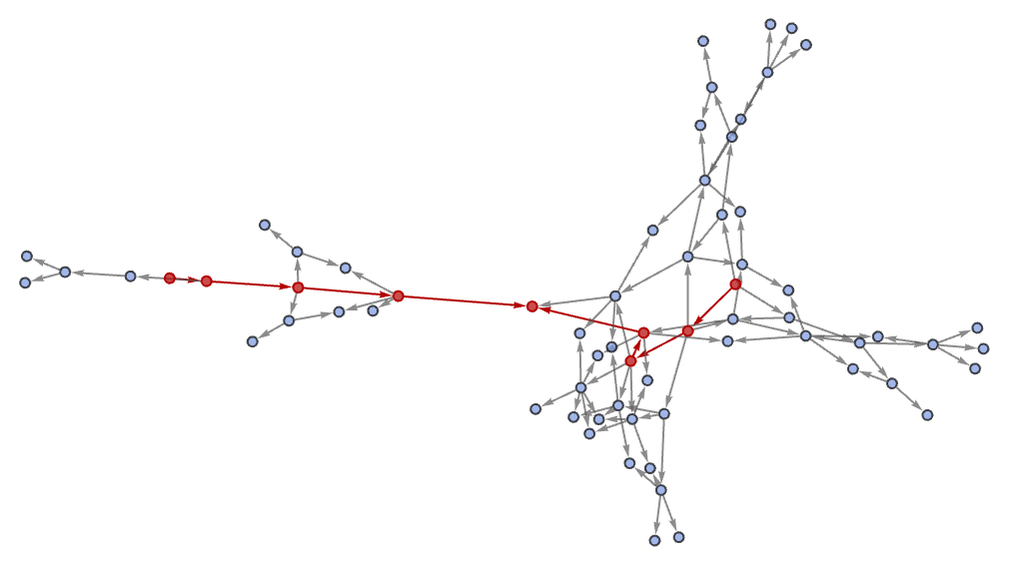
the branch pair {AAA, BAB} resolves after 4 steps. The following is essentially a proof of this:
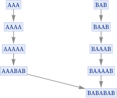
But finding this in the 67-node 4-step states graph is quite complicated:
In the rule
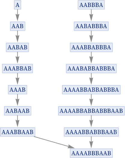
it takes 7 steps for the branch pair
to resolve to the common successor AAAABBBAAB. The 7-step states graph involved has 5869 nodes, and the proof that the branch pair resolves is:
In general, there is no upper bound on how long it may take a branch pair to resolve, or for example how long its common successor—or intermediate strings involved in reaching it—may be. Here are the simplest rules with two distinct elements that take successively longer to resolve (the last column gives the size of the states graph when resolution is found):
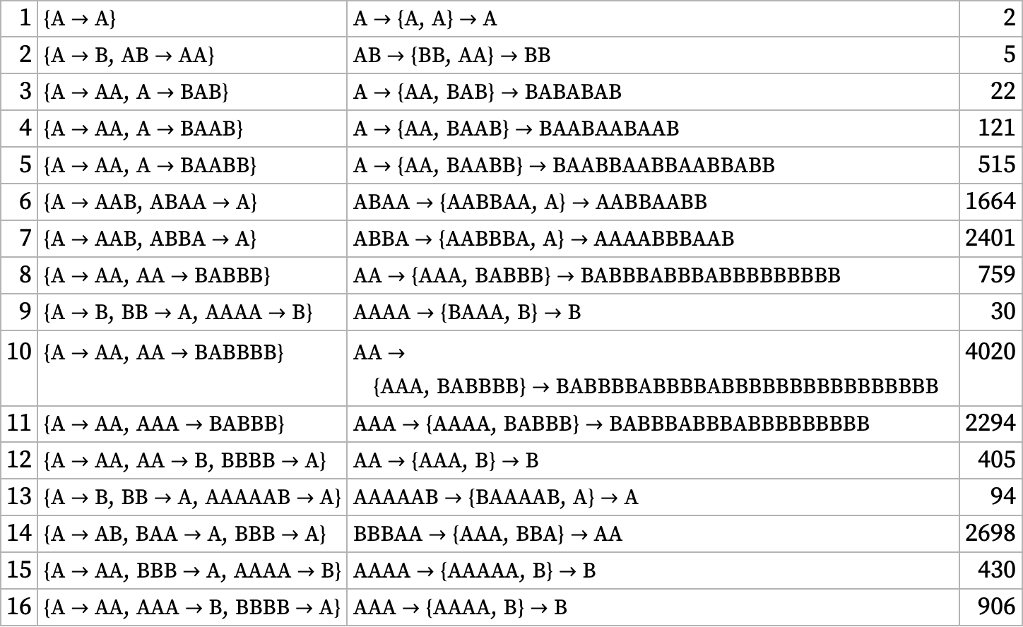
Note that—like the first case of a 2-step resolution that we showed above—quite a few of these longest-to-resolve rules actually terminate, with a member of the branch pair being their final output. Thus, for example, the last case listed is really just a reflection of the fact that with this rule, AAAA takes 16 steps to reach the termination state B:

(With 3 distinct elements similar results are seen; the first time a shorter example is seen is {A BAC, A AABA} at resolution-length 6.)
Despite the existence of long-to-resolve cases, most branch pairs in most rules in practice resolve quickly: the fraction that take τ steps seems to decrease roughly like 2–τ. But there is still in a sense an arbitrarily long tail—and the general problem of determining whether a branch pair will resolve is known to be formally undecidable (e.g. [65]).
One interesting feature of causal invariance testing is that (while still in principle undecidable) it is in some ways easier to test for total causal invariance than to test for partial causal invariance for specific initial conditions. The reason is that if a rule is going to be totally causal invariant then there is a certain core set of branch pairs that must resolve, and if all these resolve then the rule is guaranteed to be totally causal invariant. This core set of branch pairs is derived from the possible overlaps between left-hand sides of replacements, and are the successors of the minimal “unifications” of these left-hand sides, formed by minimally overlapping the strings.
Consider the rule:
The only possible overlap between the left-hand sides is A. This leads to the minimal unification AAB, which yields the branch pair {ABAA, AB}:
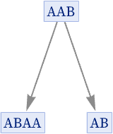
From this branch pair we construct a states graph:
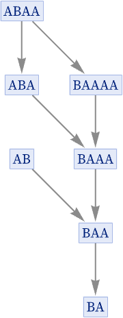
And from this we see that the branch pair resolves in 3 steps. And because this is the only branch pair that can arise through overlaps between the left-hand sides, this resolution now establishes the total causal invariance of this rule.
In the rule
there are two possible overlaps between the left-hand sides: A and B. These lead to two different minimal unifications: BAAB and ABAA. And these two unifications yield two branch pairs, {BABA, AB} and {BAAA, AA}. But now we can establish that both of these resolve, thus showing the total causal invariance of the original rule.
In general, one might in principle have to continue for arbitrarily many steps to determine if a given branch pair resolves. But the crucial point here is that because the number of possible overlaps (and therefore unifications) is fine, there are only a finite number of branch pairs one needs to consider in order to determine if a rule is totally causal invariant. There is no need to look at branch pairs that arise from larger strings than the unifications; any additional elements are basically just “padding” that cannot affect the basic interference between replacements that leads to a breakdown of causal invariance.
Looking at branch pairs from all possible unifications is a way to determine total causal invariance—and thus to determine whether a rule will be causal invariant from all possible initial conditions. But even if a rule is not totally causal invariant, it may still be causal invariant for particular initial conditions—effectively because whatever branch pairs might break causal invariance simply never occur in evolution from those initial conditions.
In practice, it is fairly common to have rules that are causal invariant for some initial conditions, but not others. In effect, there is some “conservation law” that keeps the rule away from branch pairs that would break causal invariance—and that keeps the rule operating with some subset of its possible states that happen to yield causal invariance.
 download pdf
  ARXIV
ARXIV peer review