An important consequence of causal invariance is that it establishes that a rule produces the same causal graph independent of the particular order in which update events occurred. And so this means, for example, that we can generate causal graphs just by looking at evolution with our standard updating order.
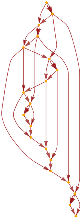
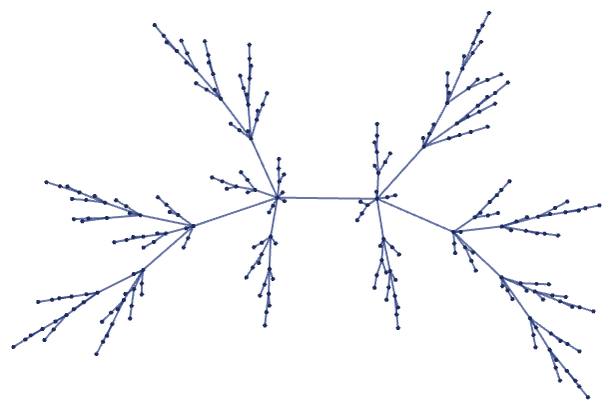
For rules that depend on only one relation, the causal graph is always just a tree
ResourceFunction[
"WolframModel"][{{x, y}} -> {{x, y}, {y, z}}, {{0, 0}}, 6,
"CausalGraph"] // LayeredGraphPlot
regardless of whether the structure generated is also a tree
ResourceFunction[
"WolframModel"][{{x, y}} -> {{x, y}, {y, z}}, {{1,
2}}, 8, "FinalStatePlot"]
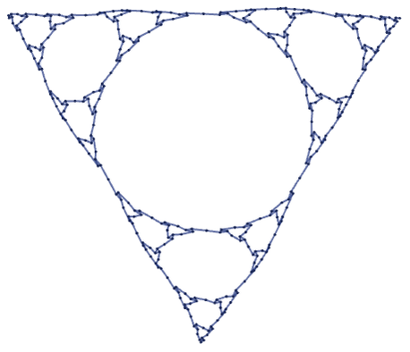
or has a more compact form:
ResourceFunction[
"WolframModel"][{{1, 2, 3}} -> {{1, 4, 6}, {2, 5, 4}, {3, 6,
5}}, {{1, 2, 3}}, 5, "FinalStatePlot"]
But as soon as a rule depends on more than one relation, the causal graph can immediately be more complicated. For example, consider even the rule:
{{x}, {x}} -> {{x}, {x}, {x}}
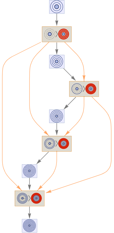
The multiway system for this rule shows that only one path is possible (immediately demonstrating causal invariance):
Graph[ResourceFunction["MultiwaySystem"][
"WolframModel" -> {{{1}, {1}} -> {{1}, {1}, {1}}}, {{{1}, {1}}}, 4,
"StatesGraph"], VertexSize -> 1]
But the causal relationships between steps are not so straightforward
CloudGet["https://wolfr.am/LmHho8Tr"]; newgraph[
ResourceFunction["MultiwaySystem"][
"WolframModel" -> {{{x}, {x}} -> {{x}, {x}, {x}}}, {{{x}, {x}}}, 4,
"EvolutionCausalGraph", VertexSize -> 1], {1, .5}]
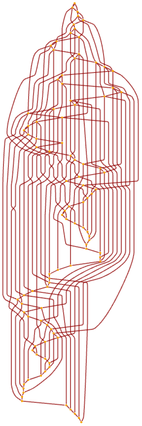
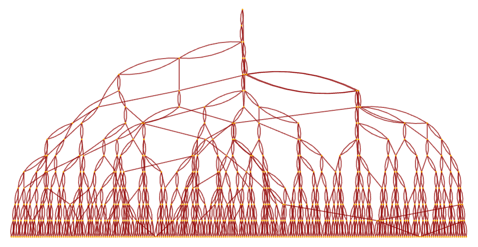
and after 15 steps the causal graph has the form
ResourceFunction[
"WolframModel"][{{x}, {x}} -> {{x}, {x}, {x}}, {{x}, {x}},
15]["LayeredCausalGraph", AspectRatio -> 1/2]
or in an alternative rendering:
ResourceFunction[
"WolframModel"][{{x}, {x}} -> {{x}, {x}, {x}}, {{x}, {x}}, 15, \
"CausalGraph"]
The fact that the multiway system is nontrivial does not mean that the causal graph for a particular rule evolution will be nontrivial. Consider for example a causal invariant rule that we discussed above:
{{x, y}, {z, y}} -> {{x, w}, {y, w}, {z, w}}
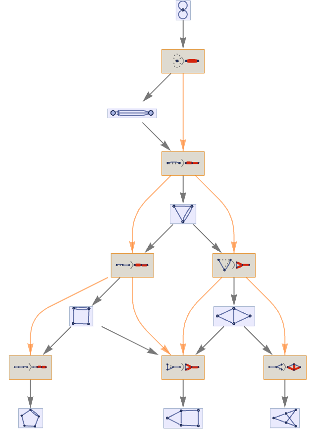
The multiway system for this rule, with causal connections shown, is:
CloudGet["https://wolfr.am/LmHho8Tr"]; newgraph[
ResourceFunction["MultiwaySystem"][
"WolframModel" -> {{{x, y}, {z, y}} -> {{x, w}, {y, w}, {z,
w}}}, {{{0, 0}, {0, 0}}}, 4, "EvolutionCausalGraph",
VertexSize -> 1], {1, .4}]
This yields the multiway causal graph:
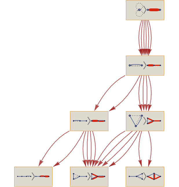
CloudGet["https://wolfr.am/LmHho8Tr"]; newgraph[
ResourceFunction["MultiwaySystem"][
"WolframModel" -> {{{x, y}, {z, y}} -> {{x, w}, {y, w}, {z,
w}}}, {{{0, 0}, {0, 0}}}, 4, "CausalGraph", VertexSize -> 1,
PerformanceGoal -> "Quality"]]
But the causal graph for any individual evolution is just:
ResourceFunction[
"WolframModel"][ {{x, y}, {z, y}} -> {{x, w}, {y, w}, {z,
w}}, {{0, 0}, {0, 0}}, 7, "CausalGraph"]
For the causal invariant rule (also discussed above)
{{x, y}, {z, y}} -> {{x, z}, {y, z}, {w, z}}
the multiway system after 5 steps has the form:
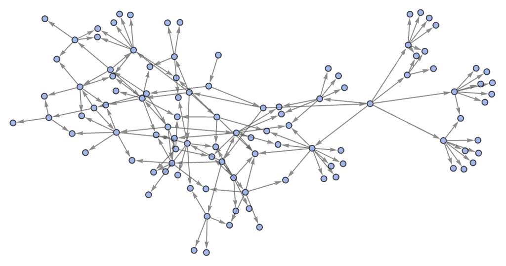
ResourceFunction["MultiwaySystem"][
"WolframModel" -> { {{x, y}, {z, y}} -> {{x, z}, {y, z}, {w,
z}}}, {{{0, 0}, {0, 0}}}, 5, "StatesGraphStructure"]
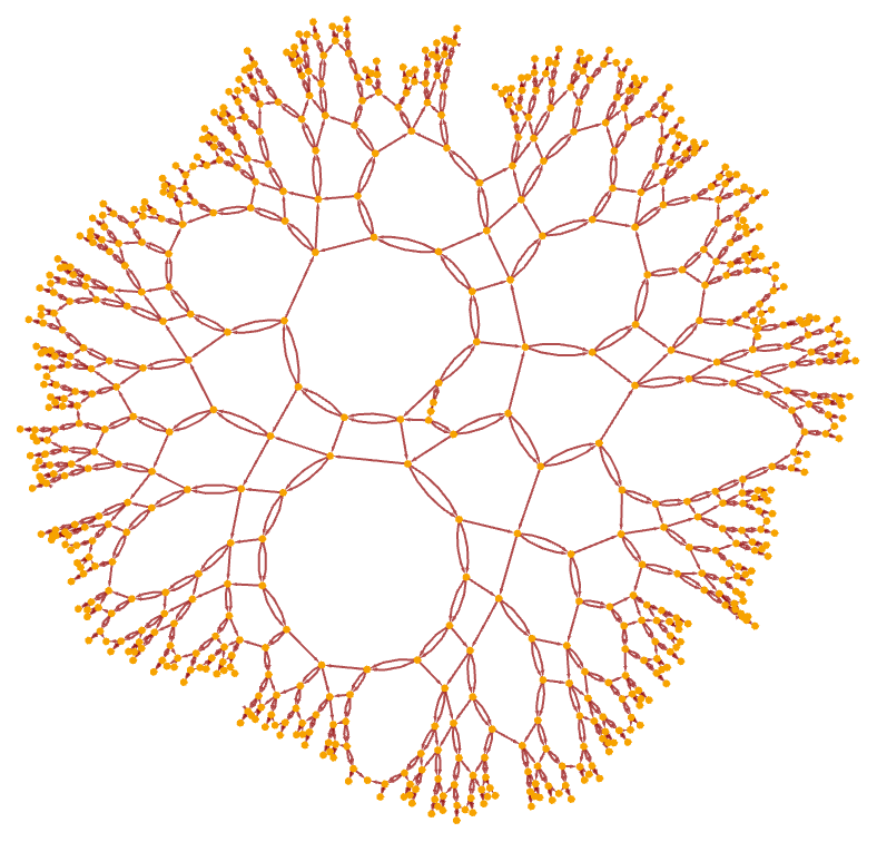
After 20 steps of evolution with our standard updating order gives:
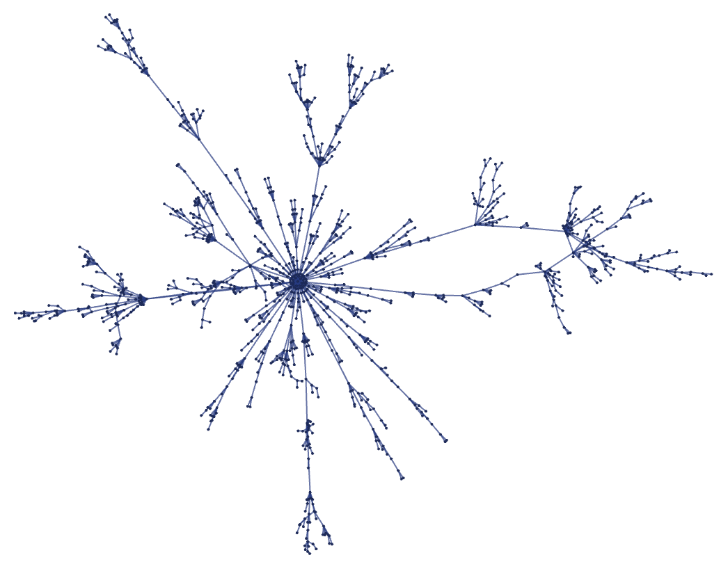
ResourceFunction[
"WolframModel"][ {{x, y}, {z, y}} -> {{x, z}, {y, z}, {w, z}}, {{0,
0}, {0, 0}}, 20, "FinalStatePlot"]
The causal graph for this rule after 10 steps is
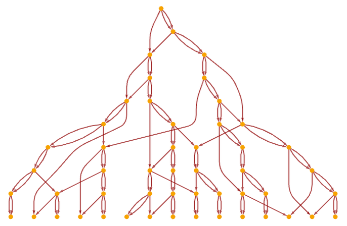
ResourceFunction[
"WolframModel"][ {{x, y}, {z, y}} -> {{x, z}, {y, z}, {w,
z}}, {{0, 0}, {0, 0}}, 10, "CausalGraph"] // LayeredGraphPlot
and after 20 steps, in a different rendering, it becomes:
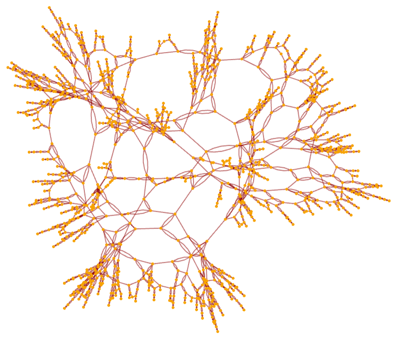
ResourceFunction[
"WolframModel"][ {{x, y}, {z, y}} -> {{x, z}, {y, z}, {w, z}}, {{0,
0}, {0, 0}}, 20, "CausalGraph"]
As another example, consider the rule (also discussed above):
{{x, y}, {x, z}} -> {{y, w}, {y, z}, {w, x}}
The multiway system for this rule (with events included) has the form:
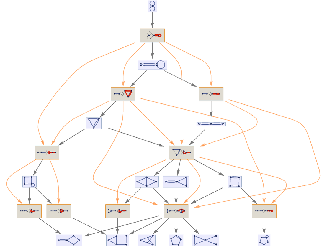
CloudGet["https://wolfr.am/LmHho8Tr"]; newgraph[
ResourceFunction["MultiwaySystem"][
"WolframModel" -> { {{x, y}, {x, z}} -> {{y, w}, {y, z}, {w,
x}}}, {{{0, 0}, {0, 0}}}, 4, "EvolutionCausalGraph",
VertexSize -> 1], {1, 0.4}]
After 20 steps, the causal graph is:
ResourceFunction[
"WolframModel"][ {{x, y}, {x, z}} -> {{y, w}, {y, z}, {w,
x}}, {{0, 0}, {0, 0}}, 20, "CausalGraph"]
After 100 steps it is:
ResourceFunction[
"WolframModel"][ {{x, y}, {x, z}} -> {{y, w}, {y, z}, {w,
x}}, {{0, 0}, {0, 0}}, 100, "LayeredCausalGraph"]
After 500 steps, in an alternative rendering, a grid-like structure emerges (the directed edges point outward from the center):
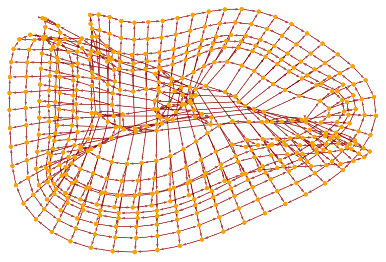
ResourceFunction[
"WolframModel"][ {{x, y}, {x, z}} -> {{y, w}, {y, z}, {w,
x}}, {{0, 0}, {0, 0}}, 500, "CausalGraph"]
After 5000 steps, rendering the graph in 3D with surface reconstruction reveals an elaborate effective geometry:
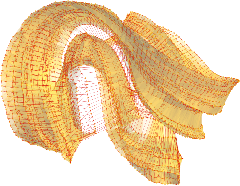
CausalGraphReconstructedSurface[w_List, delta_ : 2.5,
opts : OptionsPattern[GraphPlot3D]] :=
With[{gr = ResourceFunction["HypergraphToGraph"][w]},
Show[Graphics3D[{Hue[0.11, 1, 0.97],
Style[ResourceFunction["NonConvexHullMesh"][
GraphEmbedding[gr, "SpringElectricalEmbedding", 3], delta],
Directive[EdgeForm[], Opacity[.1]]]},
FilterRules[{opts}, Options[Graphics3D]], Boxed -> False,
BoxStyle -> Gray, Method -> {"ShrinkWrap" -> True},
Lighting -> "Neutral"],
GraphPlot3D[gr, FilterRules[{opts}, Options[GraphPlot3D]],
EdgeStyle -> {
Hue[0, 1, 0.8300000000000001]}, VertexSize -> 2,
VertexStyle -> {Directive[Hue[0.11, 1, 0.97], Opacity[.6],
EdgeForm[None]]}]]]; CausalGraphReconstructedSurface[
List @@@ EdgeList[
ResourceFunction[
"WolframModel"][ {{x, y}, {x, z}} -> {{y, w}, {y, z}, {w,
x}}, {{0, 0}, {0, 0}}, 5000, "CausalGraph"]]]