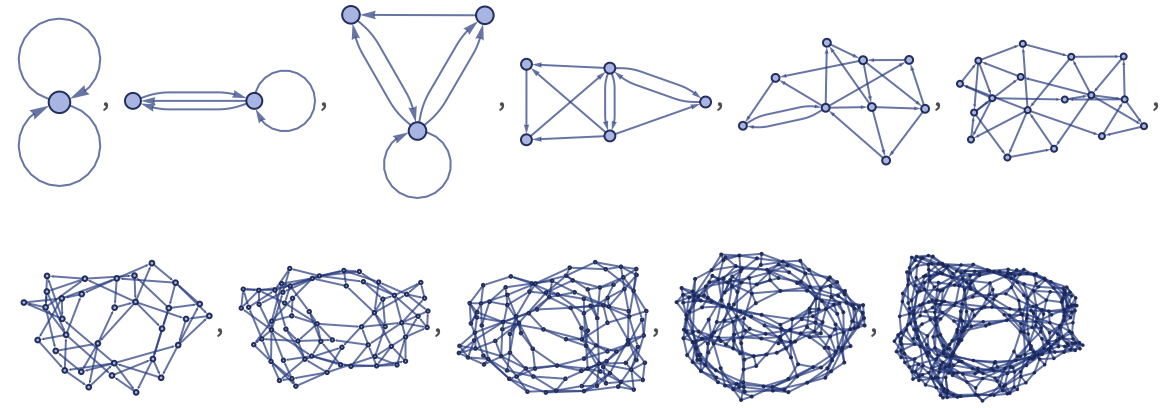
For 22 42, there are 40,405 inequivalent left-connected rules. Of these, about 36% stay connected when they evolve. Starting from two self-loops {{0,0},{0,0}}, and running for 8 steps, here is a sample of the 4000 or so distinct behaviors that are produced:
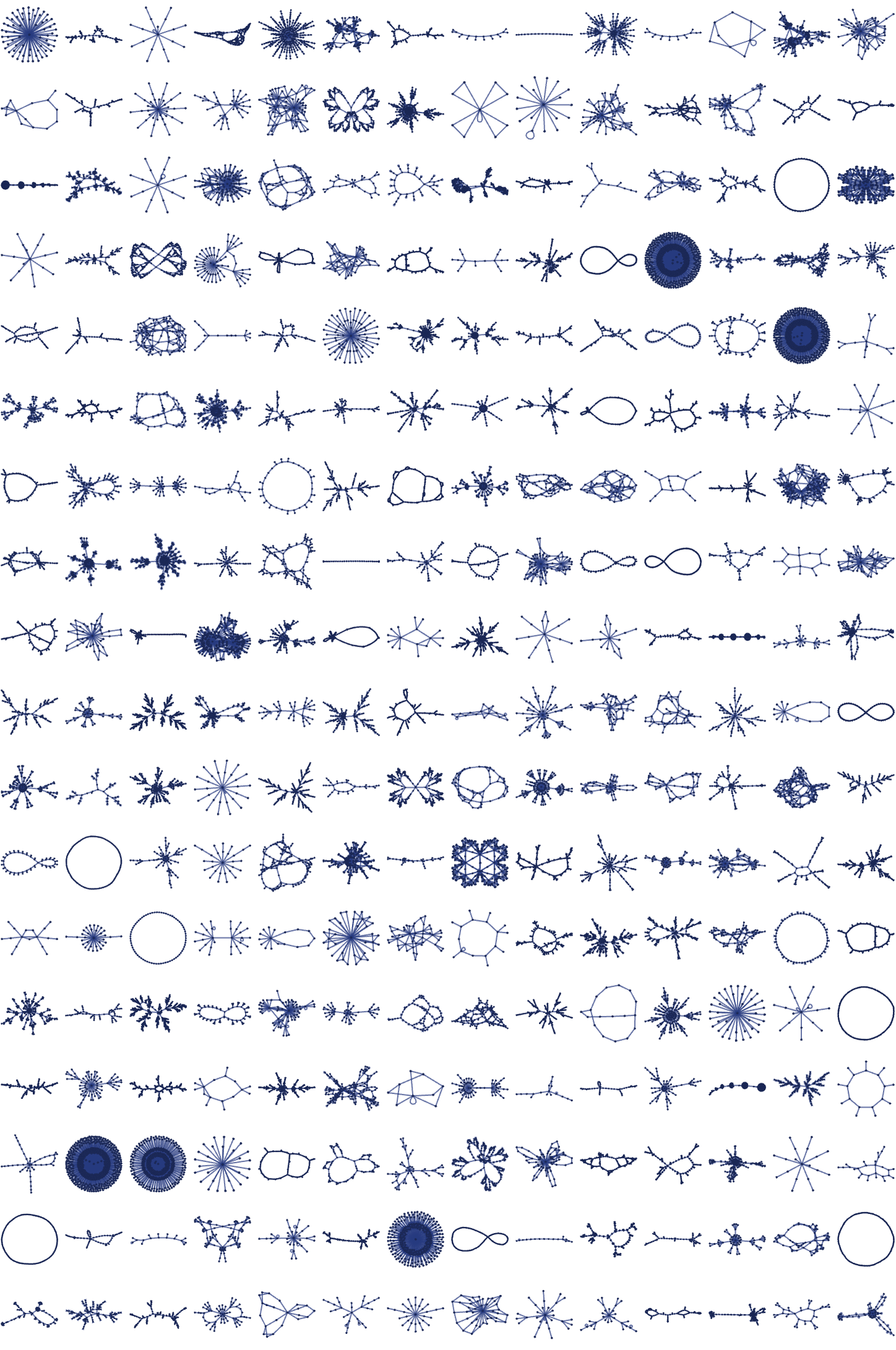
Most of these rules show the same kinds of behaviors we have seen before. But there is one major new kind of behavior that is observed: in a little less than 1% of all cases, the rules produce globular structures that in effect continually add various forms of cross-connections. Here are a few examples (notably, even though 22 42 rules can involve up to 7 distinct elements, these rules all involve just 4):
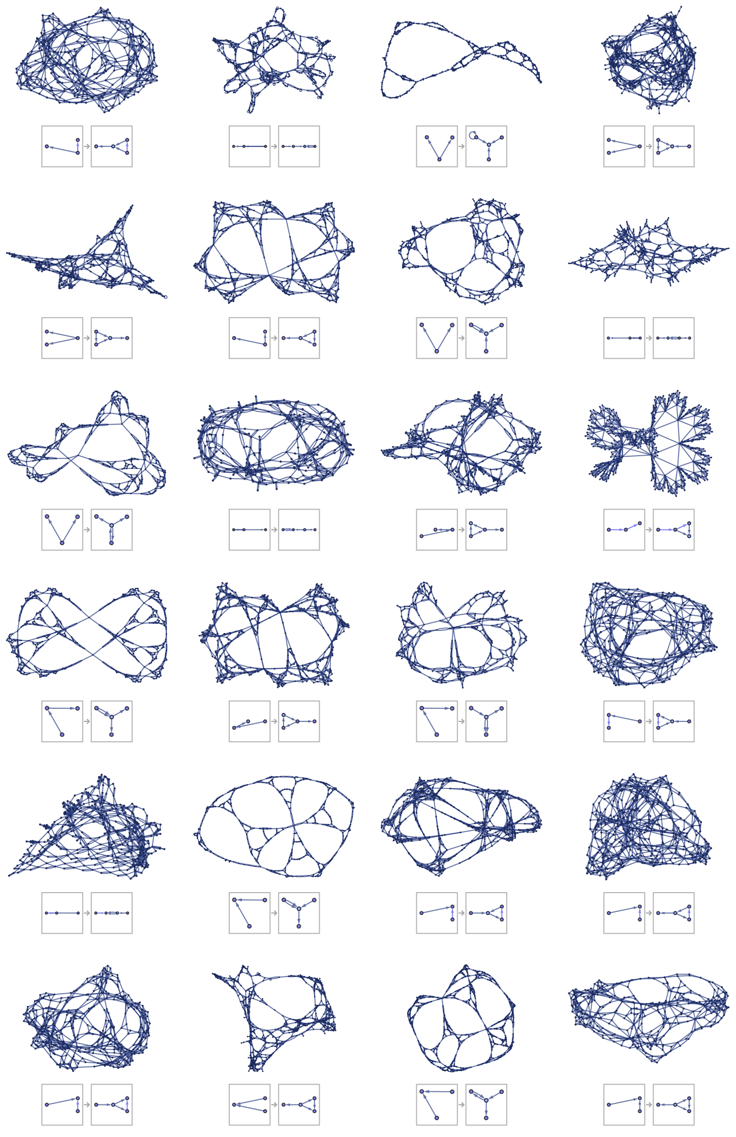
We will study these kinds of structures in more detail later. Note that the specific forms shown here depend on the underlying updating order used—though for example random orders typically seem to give similar results. It is also the case that the detailed visual layout of graphs can affect the impression of these structures; we will address this in the next section when we discuss various forms of quantitative analysis.
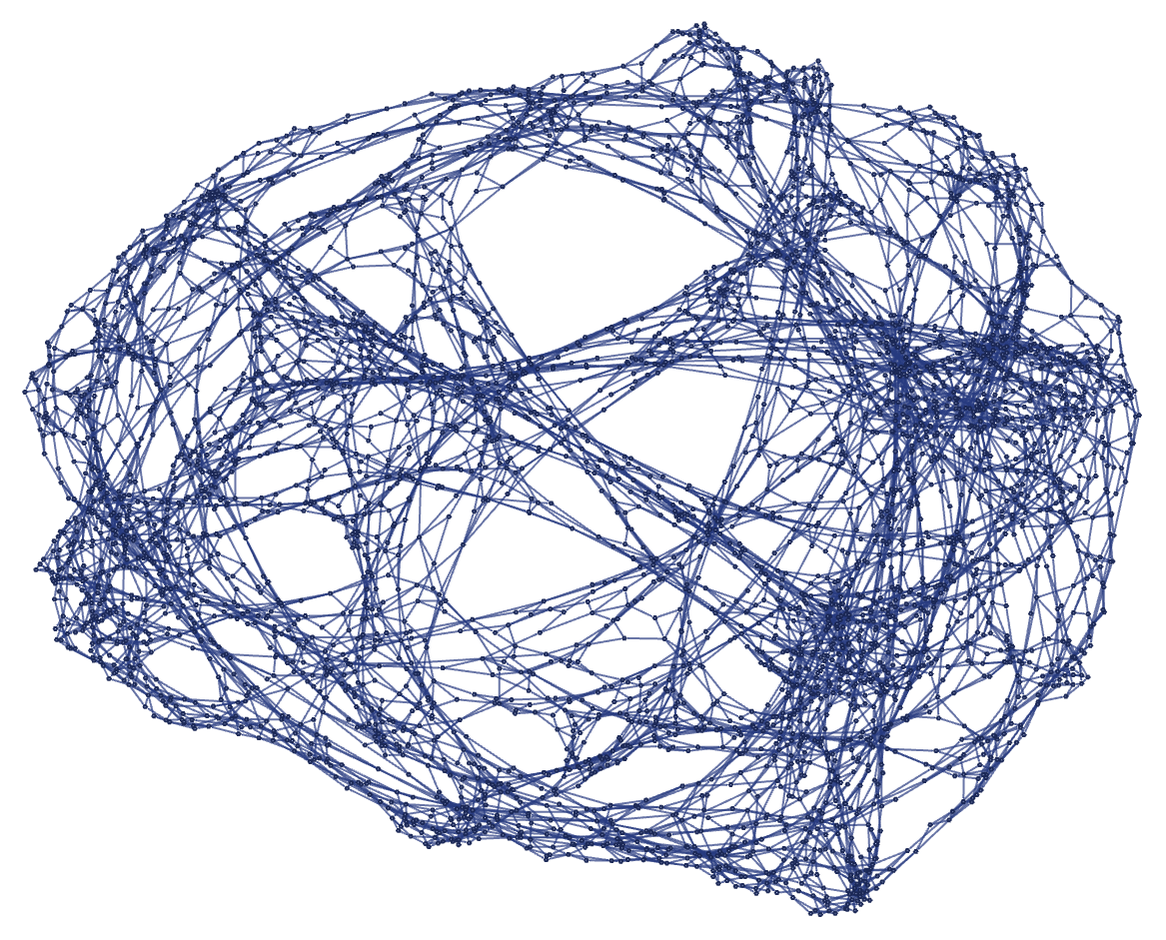
It is remarkable how complex the structures are that can be created even from very simple rules. Here are three examples (with short codes wm5583, wm4519, wm2469) shown in more detail:


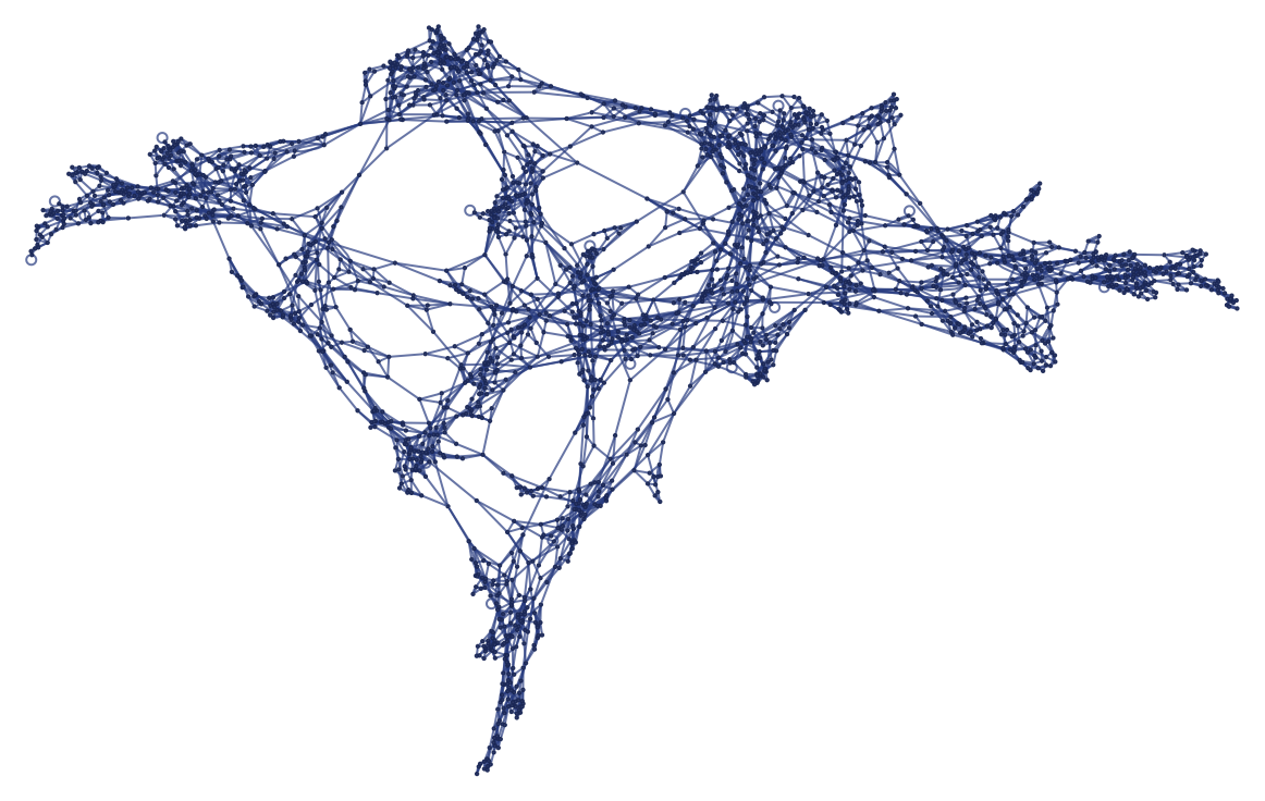


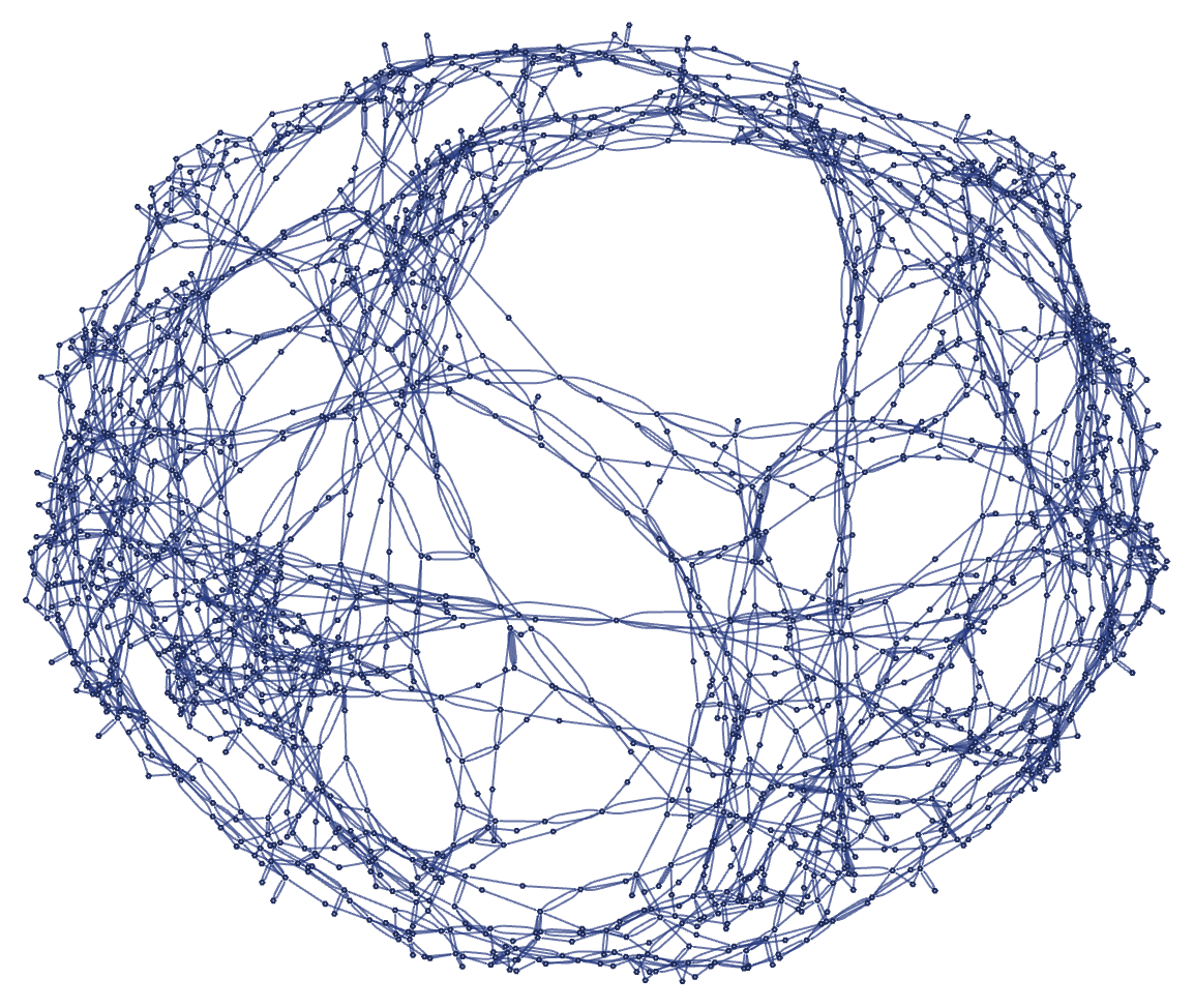

Much as we have seen in other systems such as cellular automata [1], there seems to be no simple way to deduce from the rules from our systems here what their behavior will be. And indeed even seemingly very similar rules can give dramatically different behavior, sometimes simple, and sometimes complex.
 download pdf
  ARXIV
ARXIV peer review