Our goal with the models introduced here is to have systems that are intrinsically as structureless as possible, and are therefore in a sense as flexible and general as possible. And one way to see how successful we have been is to look at what is involved in reproducing other systems using our models.
As a first example, consider the case of string substitution systems (e.g [1:3.5]). An obvious way to represent a string is to use a sequence of relations to set up what amounts to a linked list. The “payload” at each node of the linked list is an element of the string. If one has two kinds of string elements A and B, these can for example be represented respectively by 3-ary and 4-ary relations. Thus, for example, the string ABBAB could be (where the Bs can be identified from the “inner self-loops” in their 4-ary relations):

Note that the labels of the elements and the order of relations are not significant, so equivalent forms are
or, with our standard canonicalization:
A rule like
can then be translated to
or:
Starting with A, the original rule gives:
In terms of our translation, this is now:

The causal graph for the rule in effect shows the dependence of the string elements
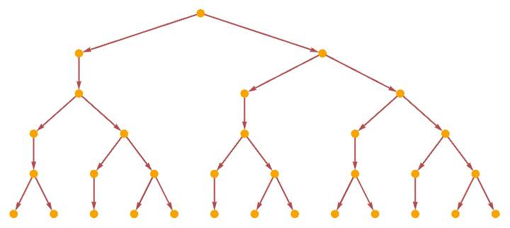
corresponding to the evolution graph (see 5.1):
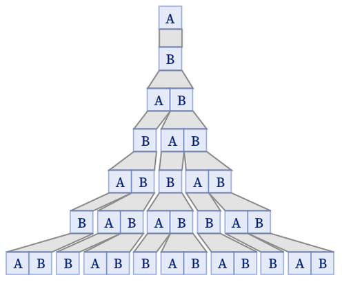
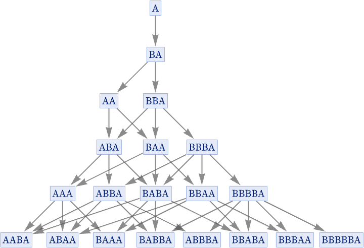
We can also take our translation of the string substitution system, and use it in a multiway system:
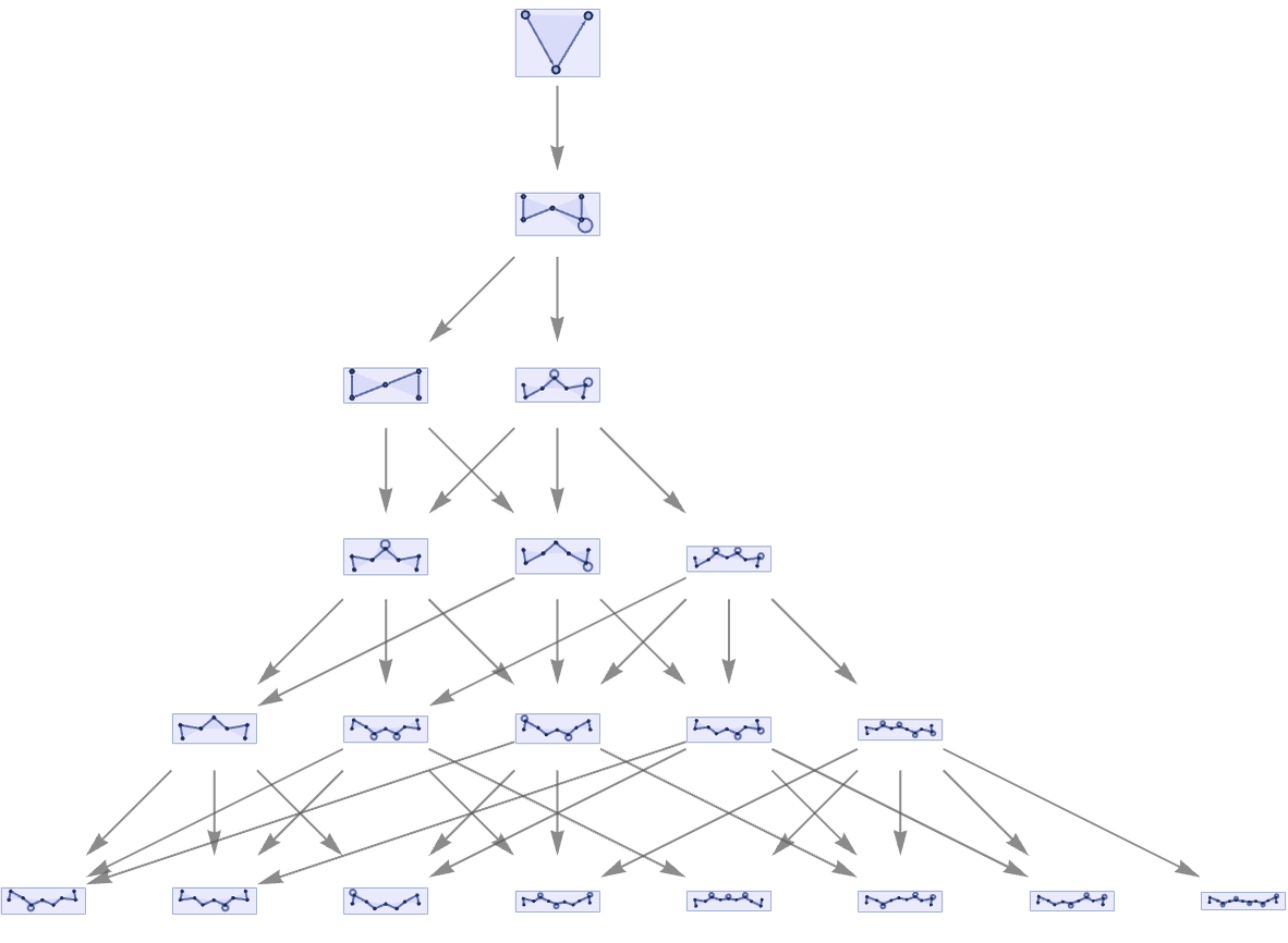
The result is a direct translation of what we could get with the underlying string system:
Having seen how our models can reproduce string substitution systems, we consider next the slightly more complex case of reproducing Turing machines [93].
As an example, consider the simplest universal Turing machine [1:p709][94][95] [96], which has the 2-state 3-color rule:

Given a tape with the Turing machine head at a certain position
a possible encoding uses different-arity hyperedges to represent different values on the tape, and different states for the head, then attaches the head to a certain position on the tape, and uses special (in this case 6-ary) hyperedges to provide “extensible end caps” to the tape:

With this setup, the rule can be encoded as:

Starting from a representation of a blank tape, the first few steps of evolution are (note that the tape is extended as needed)
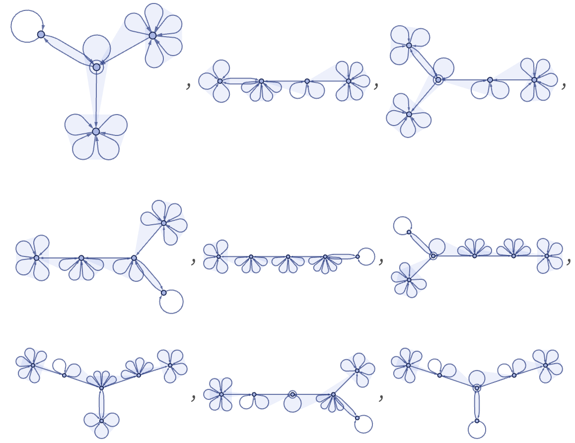
which corresponds to the first few steps of the Turing machine evolution:

The causal graph for our model directly reflects the motion of the Turing machine head, as well as the causal connections generated by symbols “remembered” on the tape between head traversals:

Re-rendering this causal graph, we see that it begins to form a grid:
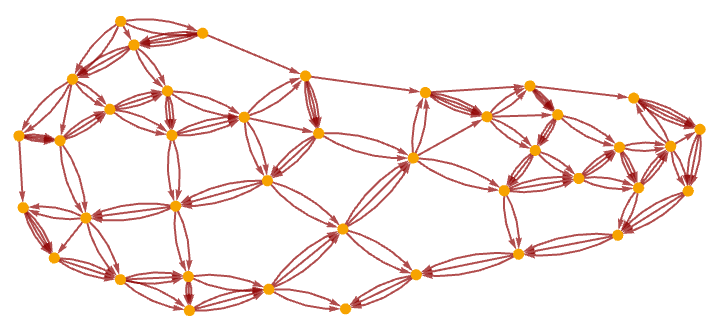
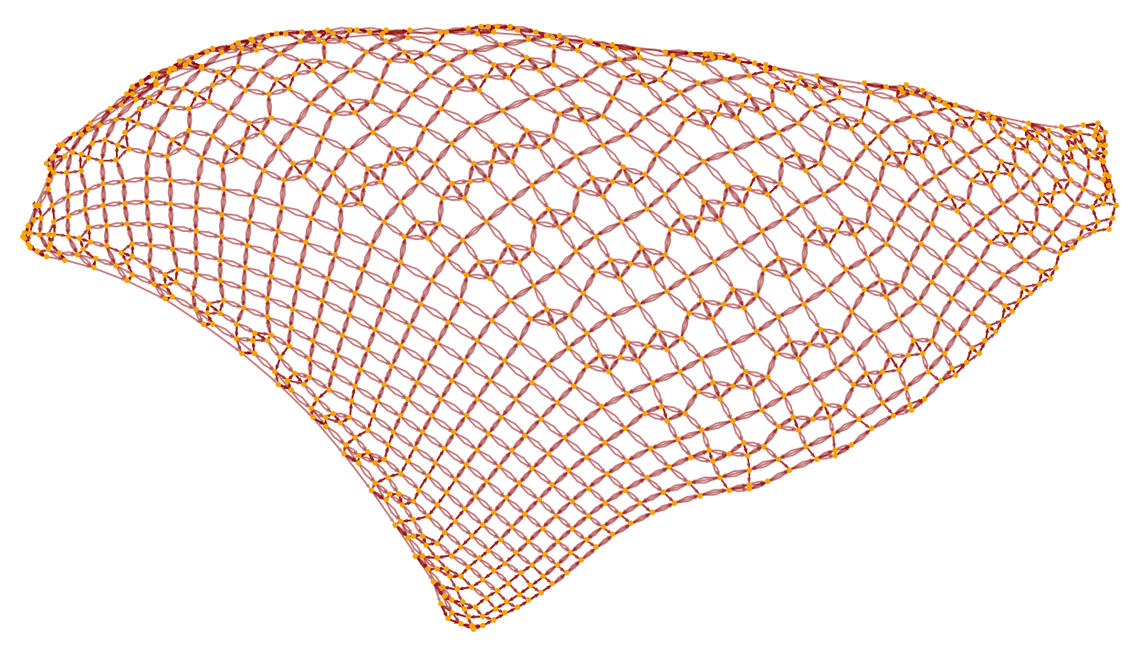
It is notable that even though in the underlying Turing machine only one action happens at each step, the causal graph still connects many events in parallel (cf. [1:p489]). After 1000 steps the graph has become a closer approximation to a flat 2D manifold, with the specific Turing machine evolution reflected in the detailed “knitting” of connections on its surface:
The rule we have set up allows only one thread of history, so the multiway system is trivial:

But with our model the underlying setup is general enough that it can handle not only ordinary deterministic Turing machines in which each possible case leads to a specific outcome, but also non-deterministic ones (as used in formulating NP problems) (e.g. [97]), in which there are multiple outcomes for some cases:

For a non-deterministic Turing machine, there can be multiple paths in the multiway system:
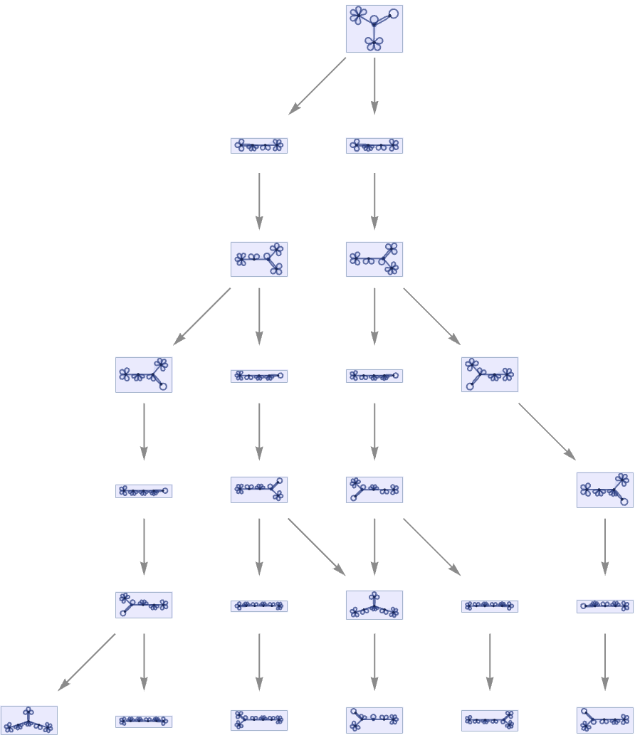
Continuing this, we see that the non-deterministic Turing machine shows a fairly complex pattern of branching and merging in the multiway system (this particular example is not causal invariant):
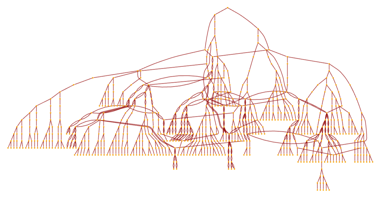
After a few more steps, and using a different rendering, the multiway system has the form:
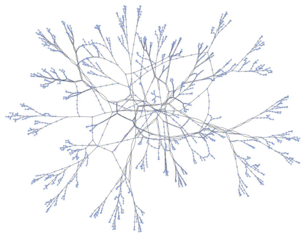
(Note that in actually using a non-deterministic Turing machine, say to solve an NP-complete problem, one needs to check the results on each branch of the multiway system—with different search strategies corresponding to using different foliations in exploring the multiway system.)
As a final example, consider using our models to reproduce cellular automata. Our models are in a sense intended to be as flexible as possible, while cellular automata have a simple but rigid structure. In particular, a cellular automaton consists of a rigid array of cells, with specific, discrete values that are updated in parallel at each step. In our models, on the other hand, there is no intrinsic geometry, no built-in notion of “values”, and different updating events are treated as independent and “asynchronous”, subject only to the partial ordering imposed by causal relations.
In reproducing a Turing machine using our models, we already needed a definite tape that encodes values, but we only had to deal with one action happening at a time, so there was no issue of synchronization. For a cellular automaton, however, we have to arrange for synchronization of updates across all cells. But as we will see, even though our models ultimately work quite differently, there is no fundamental problem in doing this with the models.
For example, given the rule 30 cellular automaton
we encode a state like
in the form

where the 6-ary self-loops represent black cells. Note that there is a quite complex structure that in effect maintains the cellular automaton array, complete with “extensible end caps” that allow it to grow.
Given this structure, the rule corresponding to the rule 30 cellular automaton becomes

where the first two transformations relate to the end caps, and the remaining 8 actually implement the various cases of the cellular automata rule. Applying the rule for our model for a few steps to an initial condition consisting of a single black cell, we get:
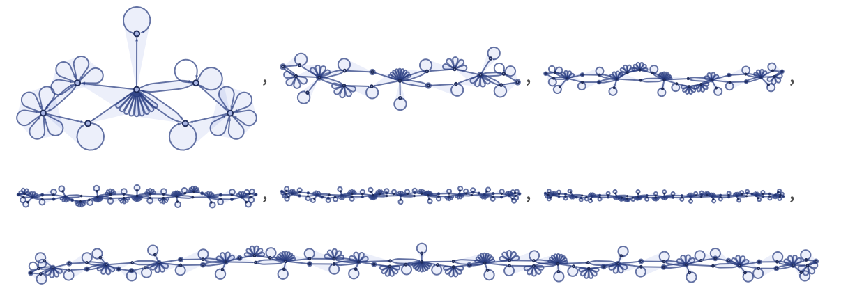
Each of these steps has information on certain cells in the cellular automaton at a certain step in the cellular automaton evolution. “Decoding” each of the steps in our model shown above, we get the following, in which the “front” of cellular automaton cells whose values are present at that step in our model are highlighted:
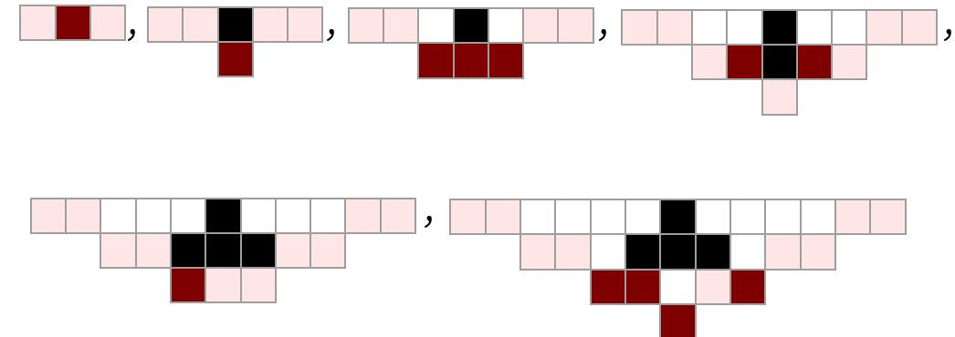
The particular foliation we have used to determine the steps in the evolution of our model corresponds to a particular foliation of the evolution of the cellular automaton:
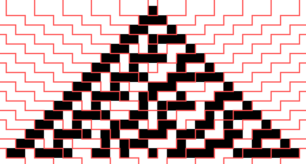
The final “spacetime” cellular automaton pattern is the same, but the foliation defines a specific order for building it up. We can visualize the way the data flows in the computation by looking at the causal graph (with events forming cells with different colors indicated):
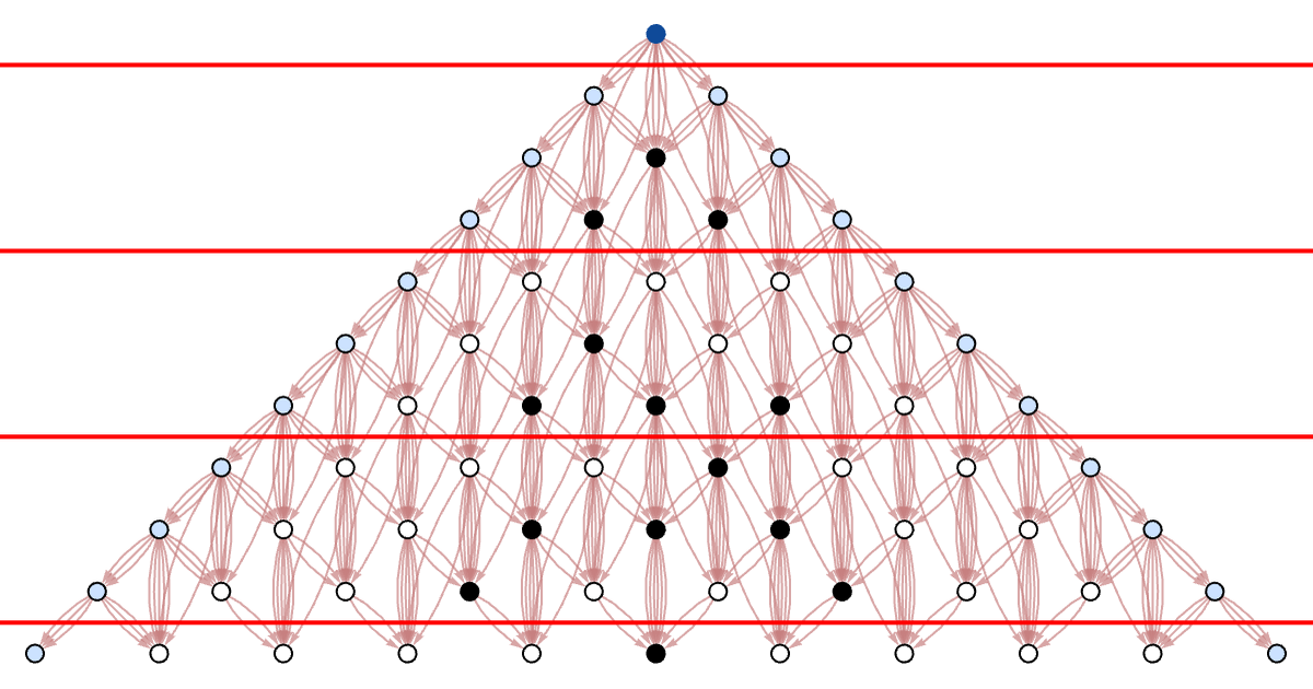
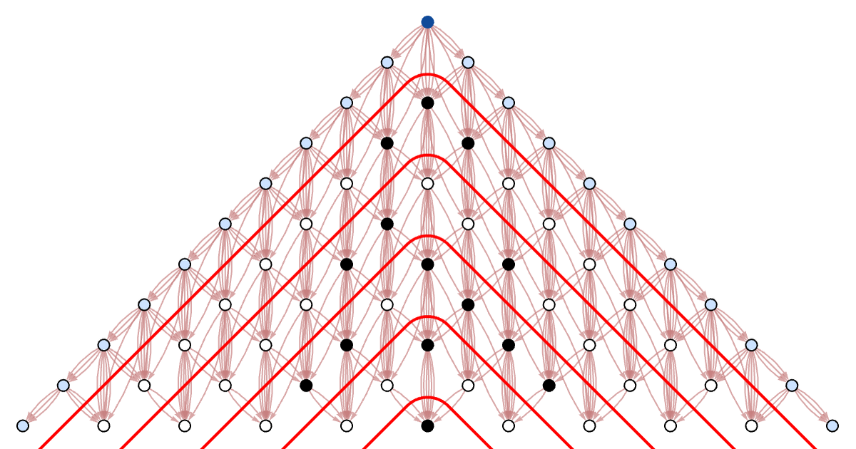
Here is the foliation of the causal graph that corresponds to each step in a traditional synchronized parallel cellular automaton updating:
 download pdf
  ARXIV
ARXIV peer review