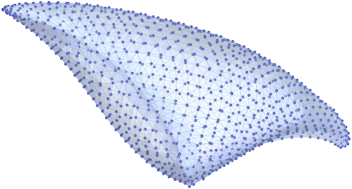
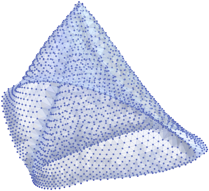
Particularly for potential applications to fundamental physics, it will be of great importance to understand what happens if we run our models for many steps—and to find ways to characterize overall behavior that emerges. Sometimes the characterization is easy. One gets a loop with progressively more links:
{{x, y}} -> {{y, z}, {z, x}}
ResourceFunction["WolframModelPlot"][#, "MaxImageSize" -> 100] & /@
ResourceFunction[
"WolframModel"][{{x, y}} -> {{y, z}, {z, x}}, {{0, 0}}, 5,
"StatesList"]
Or one gets a tree with progressively more levels of branching:
{{x}} -> {{x, y}, {y}, {y}}
Flatten[Prepend[
Take[TreePlot[ResourceFunction["HypergraphToGraph"][#], Center,
ImageSize -> 70,
VertexStyle ->
ResourceFunction["WolframPhysicsProjectStyleData"][
"SpatialGraph", "VertexStyle"],
EdgeStyle ->
ResourceFunction["WolframPhysicsProjectStyleData"][
"SpatialGraph", "EdgeLineStyle"]] & /@
ResourceFunction[
"WolframModel"][{{x}} -> {{x, y}, {y}, {y}}, {{1}}, 7,
"StatesList"] /. Arrowheads[Medium] -> Arrowheads[.09], -5],
ResourceFunction["WolframModel"][{{x}} -> {{x, y}, {y}, {y}}, {{1}},
2]["StatesPlotsList", "MaxImageSize" -> 70]]]
But what about a case like the following? Is there any way to characterize the limiting behavior here?
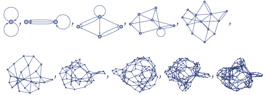
{{x, y}, {x, z}} -> {{x, y}, {x, w}, {y, w}, {z, w}}
ResourceFunction["WolframModelPlot"][#, "MaxImageSize" -> 100] & /@
ResourceFunction[
"WolframModel"][{{x, y}, {x, z}} -> {{x, y}, {x, w}, {y, w}, {z,
w}}, {{0, 0}, {0, 0}}, 9, "StatesList"]
It turns out that a rare phenomenon that we saw in the previous section gives a critical clue. Consider the rule:
{{x, y, y}, {z, x, u}} -> {{y, v, y}, {y, z, v}, {u, v, v}}
RulePlot[ResourceFunction[
"WolframModel"][{{1, 2, 2}, {3, 1, 4}} -> {{2, 5, 2}, {2, 3,
5}, {4, 5, 5}}]]
Looking at the first 10 steps it is not clear what it will do:
ResourceFunction["WolframModelPlot"][#, ImageSize -> 60] & /@
ResourceFunction[
"WolframModel"][{{1, 2, 2}, {3, 1, 4}} -> {{2, 5, 2}, {2, 3,
5}, {4, 5, 5}}, {{0, 0, 0}, {0, 0, 0}}, 10, "StatesList"]
But showing the results every 10 steps thereafter it starts to become clearer:
ResourceFunction["WolframModelPlot"][#, ImageSize -> 60] & /@
Take[ResourceFunction[
"WolframModel"][{{1, 2, 2}, {3, 1, 4}} -> {{2, 5, 2}, {2, 3,
5}, {4, 5, 5}}, {{0, 0, 0}, {0, 0, 0}}, 100, "StatesList"],
10 ;; -1 ;; 10]
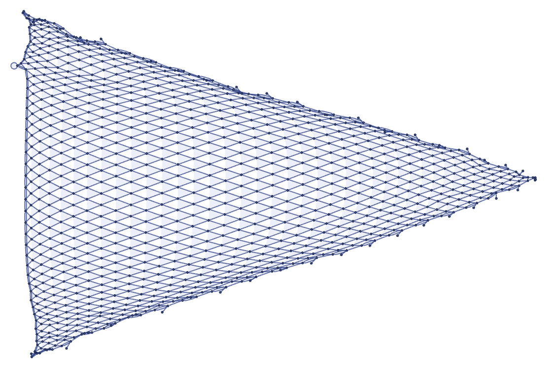
And after 1000 steps it is very clear: the rule has basically produced a simple grid:
ResourceFunction[
"WolframModel"][{{1, 2, 2}, {3, 1, 4}} -> {{2, 5, 2}, {2, 3, 5}, {4,
5, 5}}, {{0, 0, 0}, {0, 0, 0}}, 1000, "FinalStatePlot"]
Geometrical though this looks, it is important to understand that at a fundamental level there is no geometry in our model: it just involves abstract collections of relations. Our visualization methods make it evident, however, that the pattern of these relations corresponds to the pattern of connections in a grid.
In other words, from the purely combinatorial structure of the model, what we can interpret as geometrical structure has emerged. And if we continue running the model, the grid in our picture will get finer and finer, until eventually it approximates a triangular piece of continuous two-dimensional space.
Consider now the rule:
{{x, x, y}, {x, z, u}} -> {{u, u, z}, {y, v, z}, {y, v, z}}
RulePlot[ResourceFunction[
"WolframModel"][{{x, x, y}, {x, z, u}} -> {{u, u, z}, {y, v,
z}, {y, v, z}}]]
Looking at the first 10 steps of evolution it is again not clear what will happen:
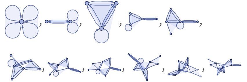
ResourceFunction["WolframModelPlot"][#, ImageSize -> 60] & /@
ResourceFunction[
"WolframModel"][{{x, x, y}, {x, z, u}} -> {{u, u, z}, {y, v,
z}, {y, v, z}}, {{0, 0, 0}, {0, 0, 0}}, 10, "StatesList"]
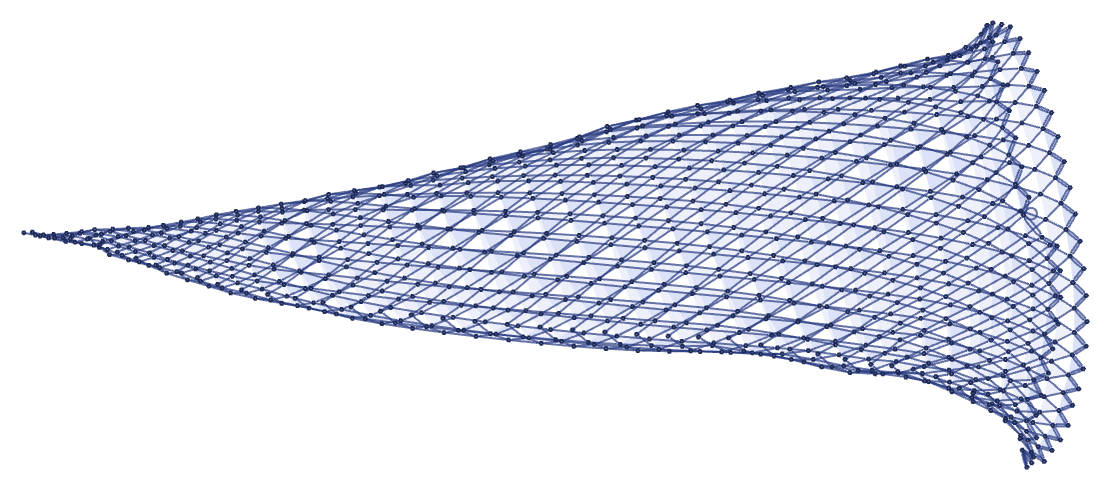
But after 1000 steps a definite geometric structure has emerged:
ResourceFunction[
"WolframModel"][{{x, x, y}, {x, z, u}} -> {{u, u, z}, {y, v, z}, {y,
v, z}}, {{0, 0, 0}, {0, 0, 0}}, 1000, "FinalStatePlot"]
There is evidence of a grid, but now it is no longer flat. Visualizing in 3D makes it clearer what is going on: the grid is effectively defining a 2D surface in 3D:
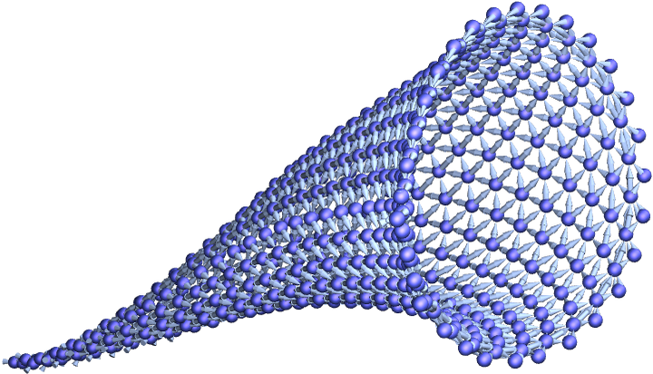
GraphPlot3D[
ResourceFunction["HypergraphToGraph"][
ResourceFunction[
"WolframModel"][{{x, x, y}, {x, z, u}} -> {{u, u, z}, {y, v,
z}, {y, v, z}}, {{0, 0, 0}, {0, 0, 0}}, 500, "FinalState"]],
VertexStyle ->
ResourceFunction["WolframPhysicsProjectStyleData"]["SpatialGraph3D",
"VertexStyle"],
EdgeStyle ->
ResourceFunction["WolframPhysicsProjectStyleData"]["SpatialGraph3D",
"EdgeLineStyle"] ]
To make its form clearer, we can go for 2000 steps, and include an approximate surface reconstruction [15]:
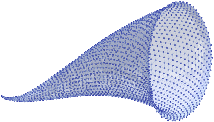
ResourceFunction["GraphReconstructedSurface"][
ResourceFunction[
"WolframModel"][{{1, 1, 2}, {1, 3, 4}} -> {{4, 4, 3}, {2, 5,
3}, {2, 5, 3}}, {{0, 0, 0}, {0, 0, 0}}, 2000, "FinalState"]]
The result is that we can identify that in the limit this rule can be characterized as creating what is essentially a cone.
Other rules produce other shapes. For example, the rule
{{x, y, z}, {u, y, v}} -> {{w, z, x}, {z, w, u}, {x, y, w}}
RulePlot[ResourceFunction[
"WolframModel"][{{x, y, z}, {u, y, v}} -> {{w, z, x}, {z, w,
u}, {x, y, w}}]]
gives after 1000 steps:
ResourceFunction[
"WolframModel"][{{1, 2, 3}, {4, 2, 5}} -> {{6, 3, 1}, {3, 6, 4}, {1,
2, 6}}, {{0, 0, 0}, {0, 0, 0}}, 1000, "FinalStatePlot"]
The structure is clearer when visualized in 3D:
ResourceFunction["GraphReconstructedSurface"][
ResourceFunction[
"WolframModel"][ {{1, 2, 3}, {4, 2, 5}} -> {{6, 3, 1}, {3, 6,
4}, {1, 2, 6}}, {{0, 0, 0}, {0, 0, 0}}, 2000, "FinalState"]]
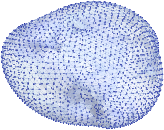
Despite its smooth form, there does not seem to be a simple mathematical characterization of this surface. (Its three-lobed structure means it cannot be an ordinary algebraic surface [16]; it is similar but not the same as the surface r = sin(ϕ) in spherical coordinates.)
Changing the initial condition from to yields the rather different surface:
ResourceFunction["GraphReconstructedSurface"][
ResourceFunction[
"WolframModel"][{{1, 2, 3}, {4, 2, 5}} -> {{6, 3, 1}, {3, 6,
4}, {1, 2, 6}}, {{0, 0, 0}, {0, 0, 0}, {0, 0, 0}}, 2000,
"FinalState"]]
This rule gives a closer approximation to a sphere, though there is a definite threefold structure to be seen:
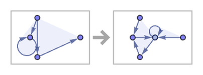
{{x, y, y}, {x, z, u}} -> {{u, v, v}, {v, z, y}, {x, y, v}}
RulePlot[ResourceFunction[
"WolframModel"][{{x, y, y}, {x, z, u}} -> {{u, v, v}, {v, z,
y}, {x, y, v}}]]
ResourceFunction["WolframModelPlot"][
ResourceFunction[
"WolframModel"][ {{x, y, y}, {x, z, u}} -> {{u, v, v}, {v, z,
y}, {x, y, v}}, {{0, 0, 0}, {0, 0, 0}}, 1000, "FinalState"]]
ResourceFunction["GraphReconstructedSurface"][
ResourceFunction[
"WolframModel"][ {{1, 2, 2}, {1, 3, 4}} -> {{4, 5, 5}, {5, 3,
2}, {1, 2, 5}}, {{0, 0, 0}, {0, 0, 0}}, 2000, "FinalState"]]
Simpler forms, such as cylindrical tubes, also appear:
{{x, x, y}, {z, u, y}} -> {{u, u, y}, {x, v, y}, {x, v, z}}
RulePlot[ResourceFunction[
"WolframModel"][{{x, x, y}, {z, u, y}} -> {{u, u, y}, {x, v,
y}, {x, v, z}}]]
ResourceFunction[
"WolframModel"][{{1, 1, 2}, {3, 4, 2}} -> {{4, 4, 2}, {1, 5, 2}, {1,
5, 3}}, {{0, 0, 0}, {0, 0, 0}}, 400, "FinalStatePlot"]
It is worth pausing for a moment to consider in what sense the limiting object here “is” a tube. What we ultimately have is a collection of relations which define a hypergraph. But there is an obvious measure of distance on the hypergraph: how many relations you have to follow to go from one element to another. So now one can ask whether there is a way to make this hypergraph distance between elements correspond to an ordinary geometrical distance. Can one assign positions in space to the elements so that the spatial distances between them agree with the hypergraph distances?
The answer in this case is that one can—by placing the elements at a lattice of positions on the surface of a cylinder in three-dimensional space. (And, conveniently, it so happens that our visualization method for hypergraphs basically automatically does this.) But it is important to realize that such a direct correspondence with an easy-to-describe surface is a rare and special feature of the particular rule used here.
Consider the rule:
{{x, x, y}, {x, z, u}} -> {{u, u, v}, {v, u, y}, {z, y, v}}
RulePlot[ResourceFunction[
"WolframModel"][{{x, x, y}, {x, z, u}} -> {{u, u, v}, {v, u,
y}, {z, y, v}}]]
After 1000 steps, this rule produces:
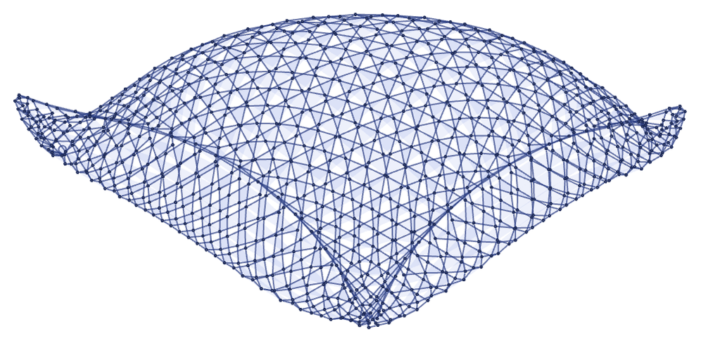
ResourceFunction[
"WolframModel"][{{1, 1, 2}, {1, 3, 4}} -> {{4, 4, 5}, {5, 4, 2}, {3,
2, 5}}, {{0, 0, 0}, {0, 0, 0}}, 1000, "FinalStatePlot"]
In 3D, this can be visualized as:
ResourceFunction["GraphReconstructedSurface"][
ResourceFunction[
"WolframModel"][{{1, 1, 2}, {1, 3, 4}} -> {{4, 4, 5}, {5, 4,
2}, {3, 2, 5}}, {{0, 0, 0}, {0, 0, 0}}, 1000, "FinalState"]]
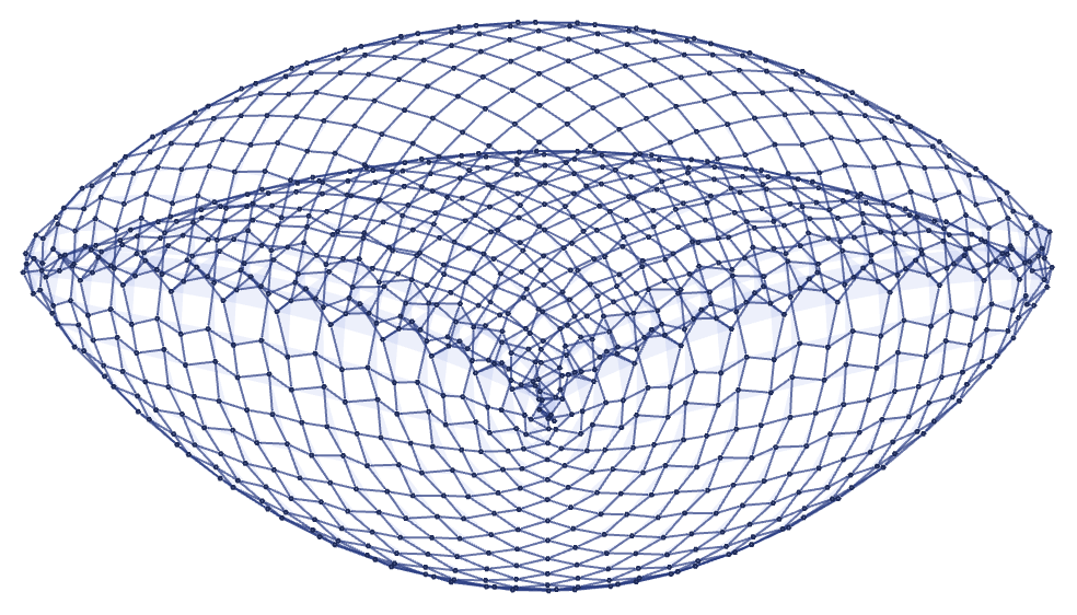
There are many subtle issues here. First, at every step the rule adds more elements, and in principle this could change the emergent geometry. But it appears that after enough steps, there is a definite limiting shape. Unlike in the case of a cylinder, however, it is much less clear how to assign spatial coordinates to different elements. It does not help that the limiting shape does not appear to have a completely smooth surface; instead there are places at which it appears to form cusps (reminiscent of an orbifold [17]).
There are rules that give more obvious “singularities”; an example is:
{{x, x, y}, {y, z, u}} -> {{v, v, u}, {v, u, x}, {z, y, v}}
RulePlot[ResourceFunction[
"WolframModel"][{{x, x, y}, {y, z, u}} -> {{v, v, u}, {v, u,
x}, {z, y, v}}]]
ResourceFunction["GraphReconstructedSurface"][
ResourceFunction[
"WolframModel"][{{1, 1, 2}, {2, 3, 4}} -> {{5, 5, 4}, {5, 4,
1}, {3, 2, 5}}, {{0, 0, 0}, {0, 0, 0}}, 2000, "FinalState"]]
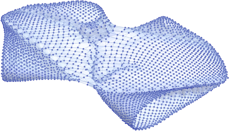
Some rules produce surfaces with complex folds:
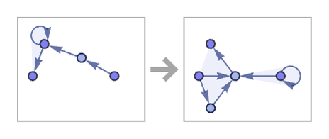
{{x, x, y}, {z, u, x}} -> {{z, z, v}, {y, v, x}, {y, w, v}}
RulePlot[ResourceFunction[
"WolframModel"][{{x, x, y}, {z, u, x}} -> {{z, z, v}, {y, v,
x}, {y, w, v}}]]
ResourceFunction["GraphReconstructedSurface"][
ResourceFunction[
"WolframModel"][{{1, 1, 2}, {3, 4, 1}} -> {{3, 3, 5}, {2, 5,
1}, {2, 6, 5}}, {{0, 0, 0}, {0, 0, 0}}, 2000, "FinalState"]]
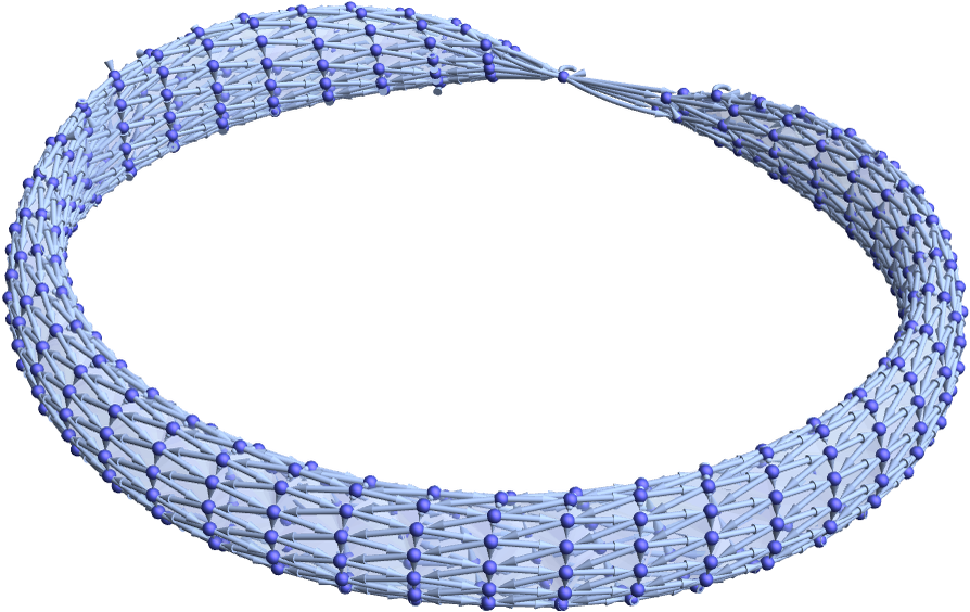
It is also perfectly possible for the emergent geometry to have nontrivial topology. This rule produces a (strangely twisted) torus:
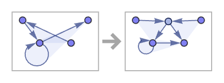
{{x, x, y}, {z, u, x}} -> {{x, x, z}, {u, v, x}, {y, v, z}}
RulePlot[ResourceFunction[
"WolframModel"][{{x, x, y}, {z, u, x}} -> {{x, x, z}, {u, v,
x}, {y, v, z}}]]
ResourceFunction["GraphReconstructedSurface"][
ResourceFunction[
"WolframModel"][{{1, 1, 2}, {3, 4, 1}} -> {{1, 1, 3}, {4, 5,
1}, {2, 5, 3}}, {{0, 0, 0}, {0, 0, 0}}, 500, "FinalState"]]
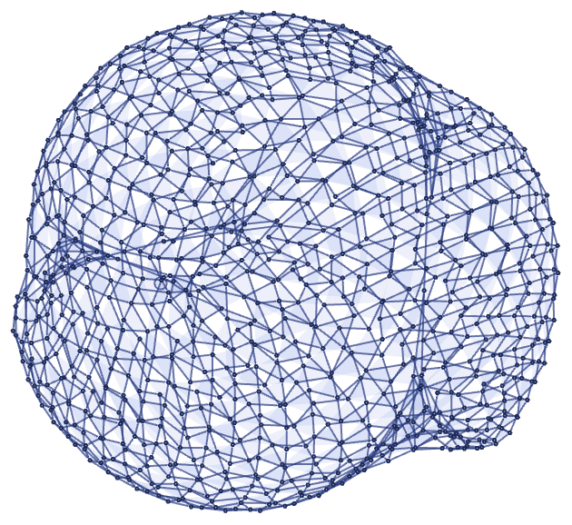
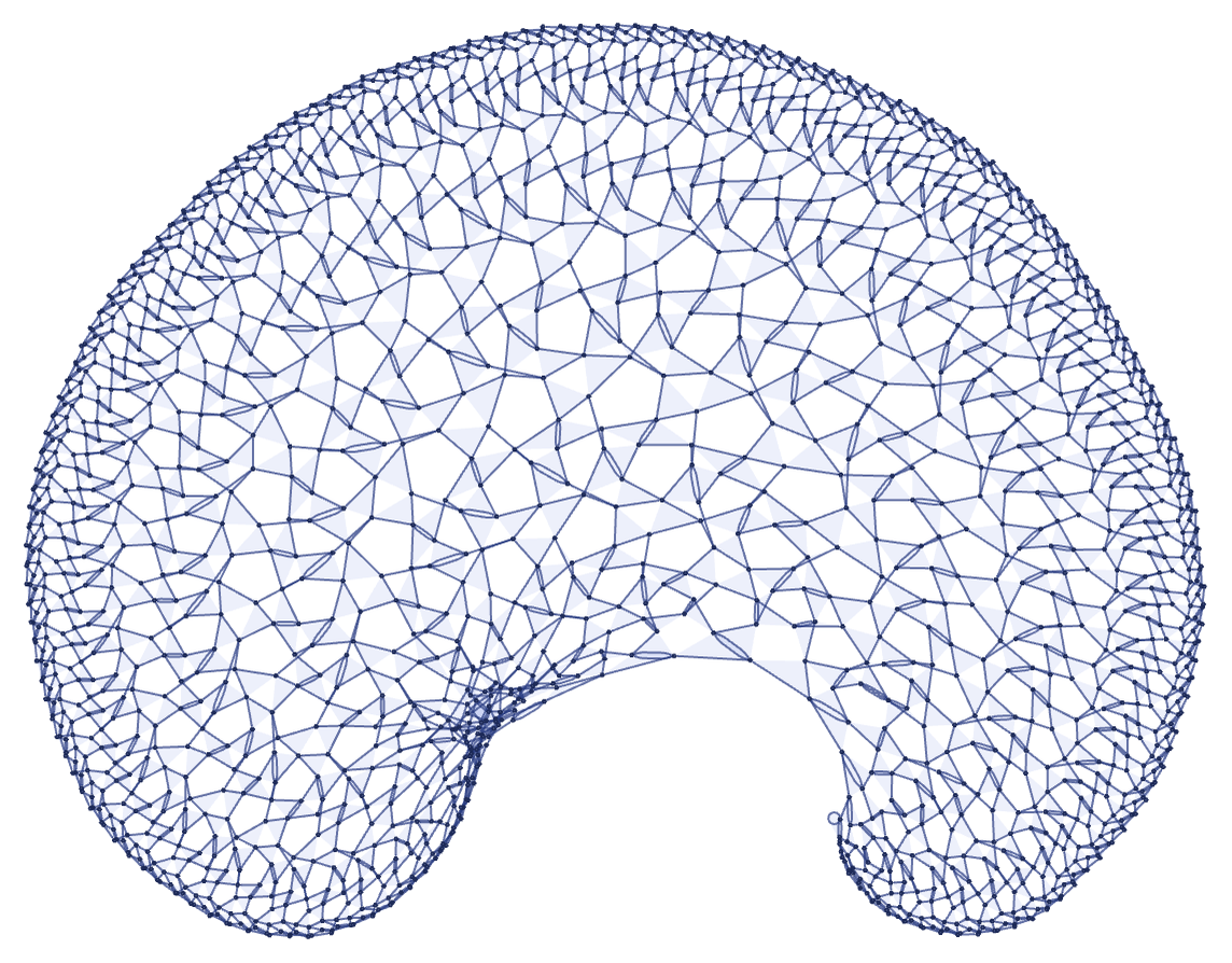
All the emergent geometries we have seen so far in effect involve a regular mesh. But this rule, instead uses a mixture of triangles, quadrilaterals and pentagons to cover a region:
{{x, y, x}, {x, z, u}} -> {{u, v, u}, {v, u, z}, {x, y, v}}
RulePlot[ResourceFunction[
"WolframModel"][{{x, y, x}, {x, z, u}} -> {{u, v, u}, {v, u,
z}, {x, y, v}}]]
ResourceFunction[
"WolframModel"][{{1, 2, 1}, {1, 3, 4}} -> {{4, 5, 4}, {5, 4, 3}, {1,
2, 5}}, {{0, 0, 0}, {0, 0, 0}}, 2000, "FinalStatePlot"]