Branchial Graphs and Multiway Causal Graphs: Wolfram Physics Project Technical Background

Consider the rule:

{{x, y}, {x, z}} -> {{x, y}, {x, w}, {y, w}, {z, w}}

If we pick a foliation for the first few steps in the multiway graph for this rule

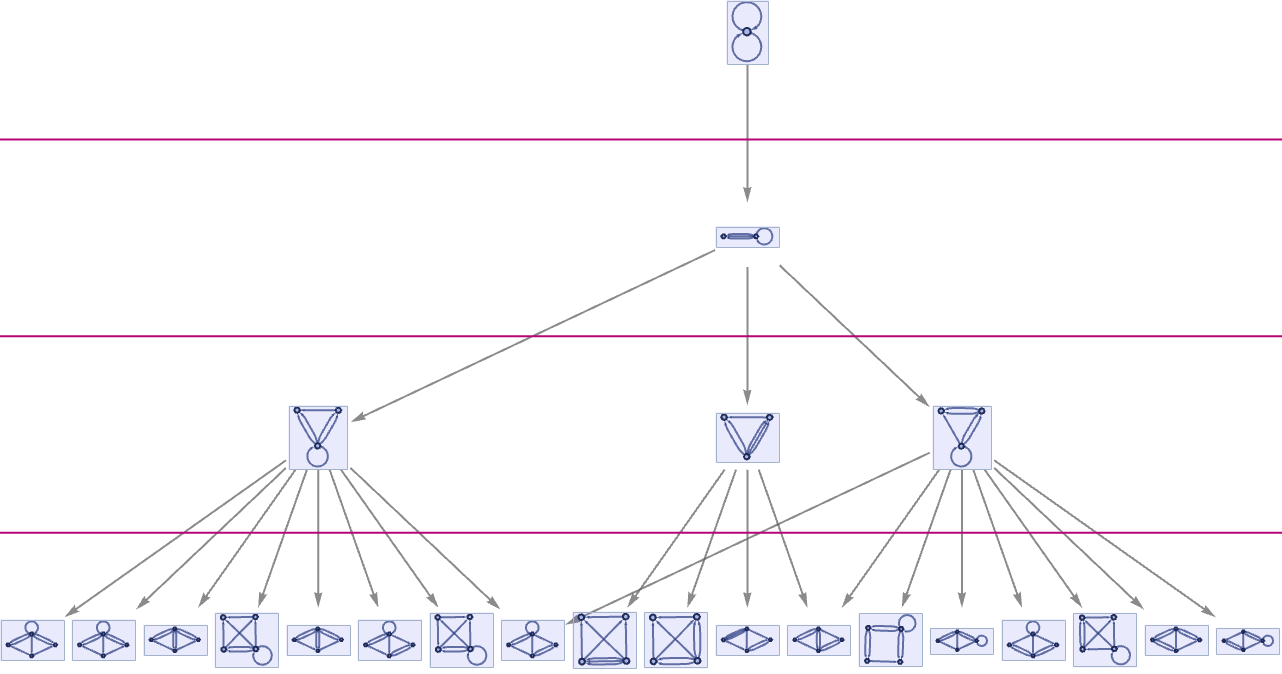
LayeredGraphPlot[ Graph[ResourceFunction["MultiwaySystem"][ "WolframModel" -> {{{x, y}, {x, z}} -> {{x, z}, {x, w}, {y, w}, {z, w}}}, {{{0, 0}, {0, 0}}}, 3, "StatesGraph"], VertexSize -> 1.8, Epilog -> {ResourceFunction["WolframPhysicsProjectStyleData"][ "BranchialGraph", "EdgeStyle"], Table[Line[{{-20, k}, {20, k}}], {k, 7, 1, -2.75}]}], AspectRatio -> 1/2]

then just as in 5.15 for string substitution systems, we can generate branchial graphs that represent the connections defined by branch pairs between the states at each slice in the foliation:

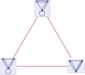
Graph[ResourceFunction["MultiwaySystem"][ "WolframModel" -> {{{x, y}, {x, z}} -> {{x, z}, {x, w}, {y, w}, {z, w}}}, {{{0, 0}, {0, 0}}}, 2, "BranchialGraph"], VertexSize -> .5]

Graph[ResourceFunction["MultiwaySystem"][ "WolframModel" -> {{{x, y}, {x, z}} -> {{x, z}, {x, w}, {y, w}, {z, w}}}, {{{0, 0}, {0, 0}}}, 3, "BranchialGraph"], VertexSize -> 1.8]

Graph[ResourceFunction["MultiwaySystem"][ "WolframModel" -> {{{x, y}, {x, z}} -> {{x, z}, {x, w}, {y, w}, {z, w}}}, {{{0, 0}, {0, 0}}}, 4, "BranchialGraph"], VertexSize -> 1]

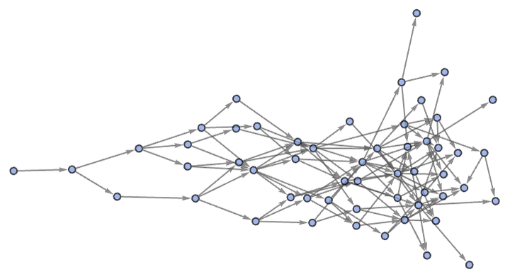
Branchial graphs provide one form of summary of the multiway evolution. Another summary is provided by the multiway causal graph, which includes causal connections between parts of hypergraphs both within a branch of the multiway system, and across different branches:

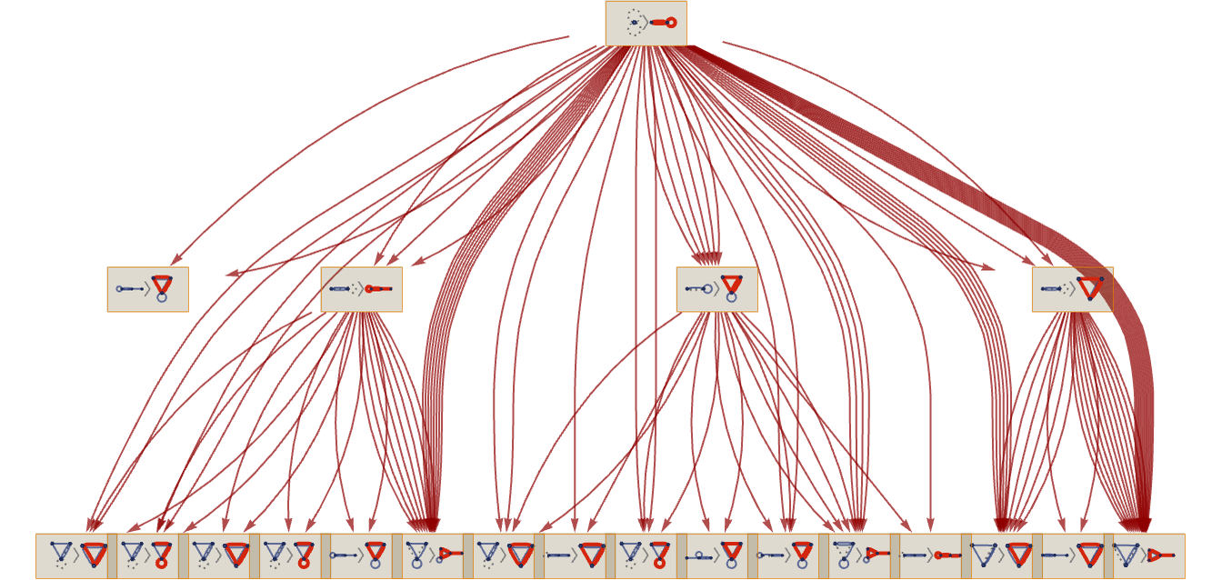
LayeredGraphPlot[ Graph[ResourceFunction["MultiwaySystem"][ "WolframModel" -> {{{x, y}, {x, z}} -> {{x, z}, {x, w}, {y, w}, {z, w}}}, {{{0, 0}, {0, 0}}}, 3, "CausalGraph"], VertexSize -> 1.8 {0.9972222222222222`, 0.29916666666666664`}], AspectRatio -> 1/2]

The multiway causal graph is in many respects the richest summary of the behavior of our models, and it will be important in our discussion of possible connections to physics.

In a case like the rule shown, the structure of branchial and multiway causal graphs is quite complex. As a simpler example, consider the causal invariant rule:

{{x, y}} -> {{x, y}, {y, z}}

ResourceFunction[ "WolframModel"][{{x, y}} -> {{x, y}, {y, z}}, {{0, 0}}, 6]["StatesPlotsList", ImageSize -> {70, UpTo[40]}]

With this rule, the multiway graph has the form:

CloudGet["https://wolfr.am/LmHho8Tr"]; newgraph[ ResourceFunction["MultiwaySystem"][ "WolframModel" -> {{{x, y}} -> {{x, y}, {y, z}}}, {{{0, 0}}}, 5, "StatesGraph", VertexSize -> 1], {1, .4}]

After more steps, and with a different rendering, the multiway graph is:

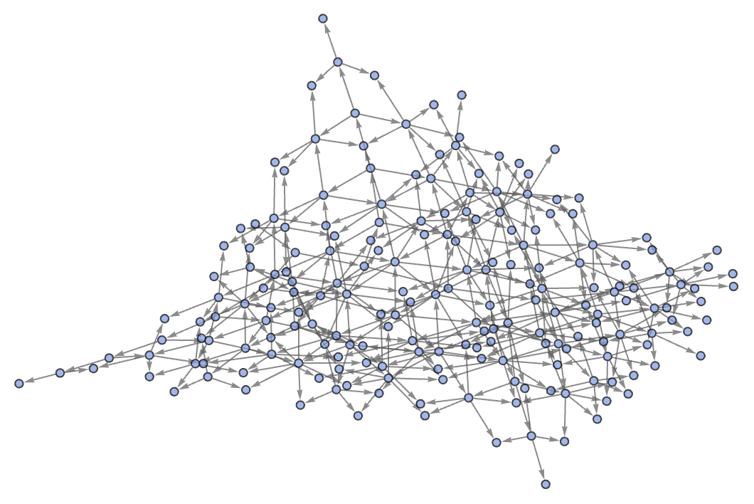
ResourceFunction["MultiwaySystem"][ "WolframModel" -> {{{x, y}} -> {{x, y}, {y, z}}}, {{{0, 0}}}, 7, "StatesGraphStructure"]

(In this case, the size of the multiway graph as measured by Σ_t increases slightly faster than 2^t.)

The branchial graphs with the standard layered foliation in this case are:

Table[Graph[ ResourceFunction["MultiwaySystem"][ "WolframModel" -> {{{x, y}} -> {{x, y}, {y, z}}}, {{{0, 0}}}, t, "BranchialGraphStructure"], ImageSize -> Tiny], {t, 2, 6}]

The volumes B_t in the branchial graph grow on successive steps like:

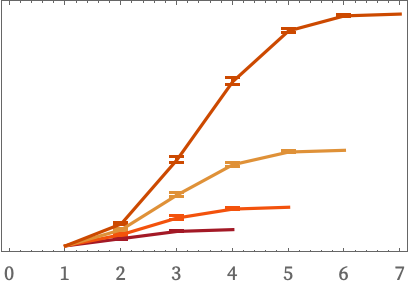
ListLinePlot[ Table[ResourceFunction["RaggedMeanAround"][ Values[ResourceFunction["GraphNeighborhoodVolumes"][ ResourceFunction["MultiwaySystem"][ "WolframModel" -> {{{x, y}} -> {{x, y}, {y, z}}}, {{{0, 0}}}, t, "BranchialGraphStructure"]]]], {t, 4, 7}], Frame -> True, FrameTicks -> {Automatic, None}, PlotStyle -> {Hue[0.9849884156577183, 0.844661839156126, 0.63801], Hue[0.05, 0.9493847125498949, 0.954757], Hue[ 0.0889039442504032, 0.7504362741954692, 0.873304], Hue[ 0.06, 1., 0.8], Hue[0.12, 1., 0.9], Hue[0.08, 1., 1.], Hue[ 0.98654716551403, 0.6728487861309527, 0.733028], Hue[ 0.04, 0.68, 0.9400000000000001], Hue[ 0.9945149844324427, 0.9892162267509705, 0.823529], Hue[ 0.9908289627180552, 0.4, 0.9]}]

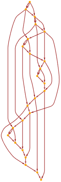
The multiway causal graph in this case is

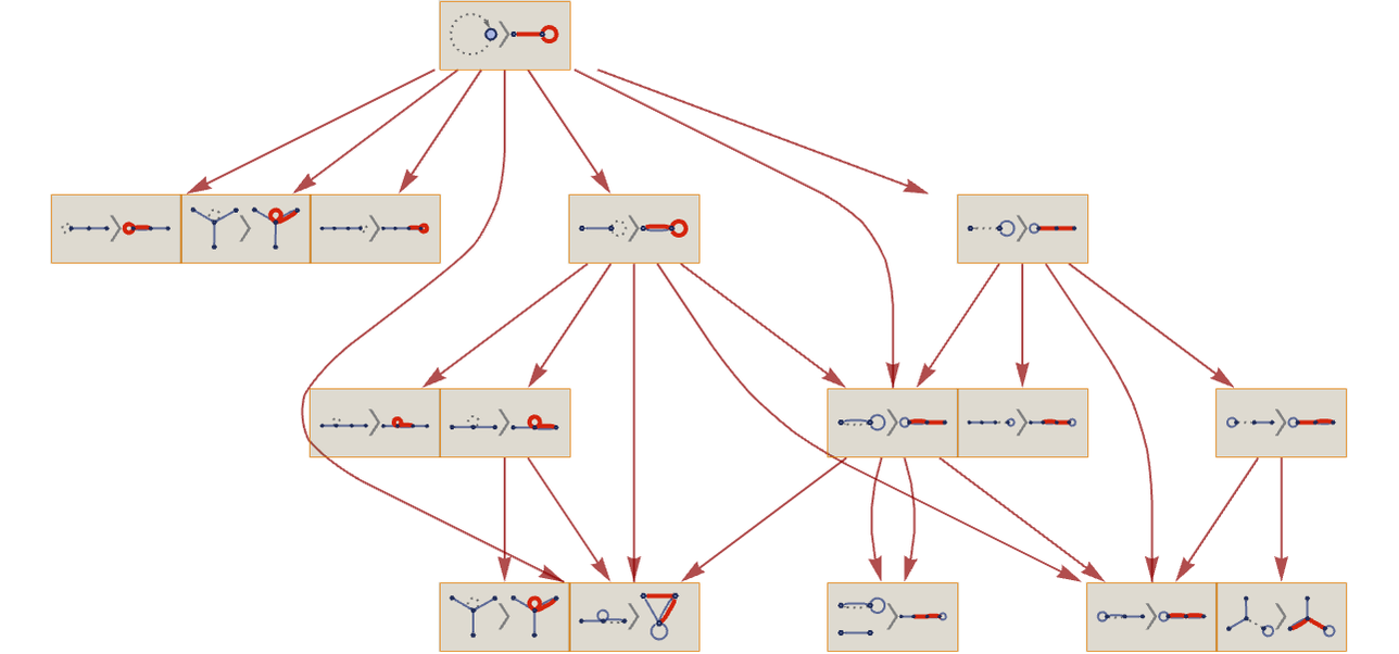
LayeredGraphPlot[ Graph[ResourceFunction["MultiwaySystem"][ "WolframModel" -> {{{x, y}} -> {{x, y}, {y, z}}}, {{{0, 0}}}, 4, "CausalGraph"], VertexSize -> 1.5 {0.9972222222222222`, 0.29916666666666664`}, AspectRatio -> 1/2]]

or with more steps and a different layout:

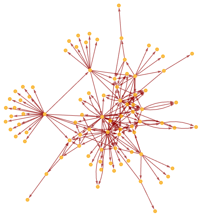
Graph[ResourceFunction["MultiwaySystem"][ "WolframModel" -> {{{x, y}} -> {{x, y}, {y, z}}}, {{{0, 0}}}, 6, "CausalGraphStructure"], GraphLayout -> "SpringElectricalEmbedding"]

Note that in this case the ordinary multiway graph is simply:

ResourceFunction[ "WolframModel"][{{x, y}} -> {{x, y}, {y, z}}, {{0, 0}}, 5, "CausalGraph"]

As a slightly more complicated example, consider the causal invariant 2₂  3₂ rule:

{{x, y}, {x, z}} -> {{y, w}, {y, z}, {w, x}}

ResourceFunction[ "WolframModel"][{{x, y}, {x, z}} -> {{y, w}, {y, z}, {w, x}}, {{0, 0}, {0, 0}}, 15]["StatesPlotsList", ImageSize -> {70, UpTo[40]}]

The multiway system in this case has the form:

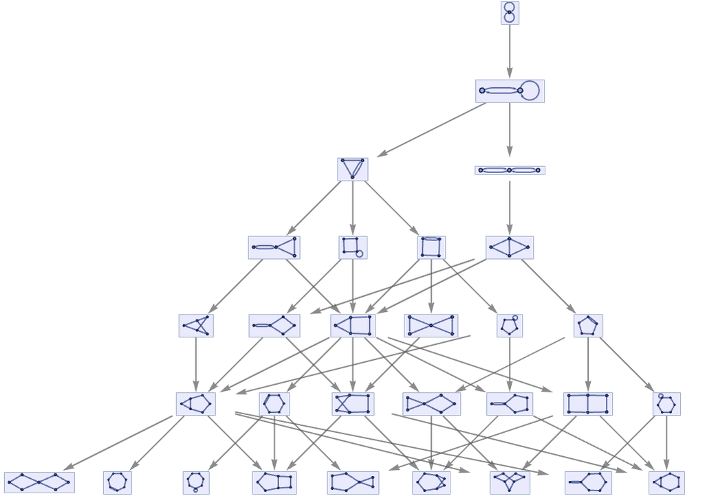
CloudGet["https://wolfr.am/LmHho8Tr"]; newgraph[ Graph[ResourceFunction["MultiwaySystem"][ "WolframModel" -> { {{x, y}, {x, z}} -> {{y, w}, {y, z}, {w, x}}}, {{{0, 0}, {0, 0}}}, 6, "StatesGraph"], VertexSize -> 1]]

ResourceFunction["MultiwaySystem"][ "WolframModel" -> {{{x, y}, {x, z}} -> {{y, w}, {y, z}, {w, x}}}, {{{0, 0}, {0, 0}}}, 8, "StatesGraphStructure"]

The sequence of branchial graphs in this case are:

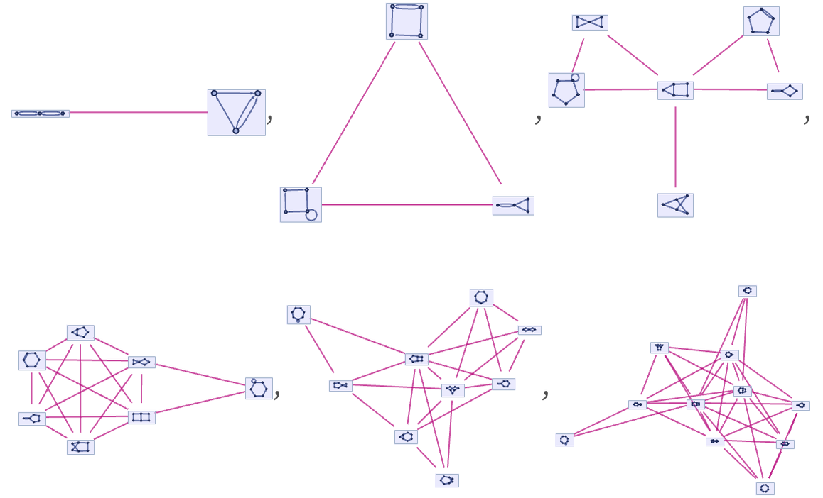
Table[Graph[ ResourceFunction["MultiwaySystem"][ "WolframModel" -> {{{x, y}, {x, z}} -> {{y, w}, {y, z}, {w, x}}}, {{{0, 0}, {0, 0}}}, t, "BranchialGraph"], VertexSize -> ({1, .6, .4, 1, 1, 1, 1, 1}[[t]])], {t, 2, 7}]

The causal graph for this rule is:

ResourceFunction[ "WolframModel"][ {{x, y}, {x, z}} -> {{y, w}, {y, z}, {w, x}}, {{0, 0}, {0, 0}}, 25, "CausalGraph"]

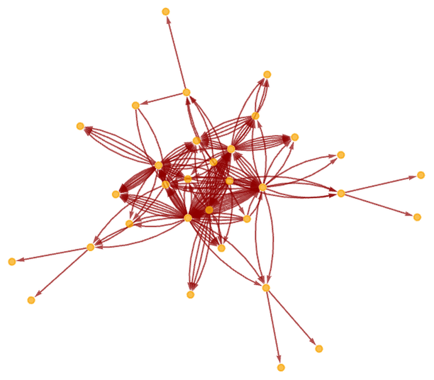
The multiway causal graph has many repeated edges:

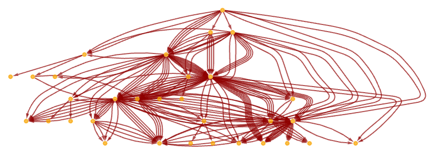
Graph[ResourceFunction["MultiwaySystem"][ "WolframModel" -> { {{x, y}, {x, z}} -> {{y, w}, {y, z}, {w, x}}}, {{{0, 0}, {0, 0}}}, 7, "CausalGraphStructure"]]

Here it is in a different rendering:

Graph[ResourceFunction["MultiwaySystem"][ "WolframModel" -> { {{x, y}, {x, z}} -> {{y, w}, {y, z}, {w, x}}}, {{{0, 0}, {0, 0}}}, 7, "CausalGraphStructure"], GraphLayout -> "SpringElectricalEmbedding"]

Note that in our models, even when the hypergraphs are disconnected, the branchial graphs can still be connected, as in the case of the rule:

{{x, y}} -> {{y, z}, {z, w}}

ResourceFunction[ "WolframModel"][{{1, 2}} -> {{2, 3}, {3, 4}}, {{0, 0}}, 6]["StatesPlotsList", ImageSize -> {70, UpTo[40]}]

Table[Graph[ ResourceFunction["MultiwaySystem"][ "WolframModel" -> {{{1, 2}} -> {{2, 3}, {3, 4}}}, {{{0, 0}}}, t, "BranchialGraphStructure"], ImageSize -> Tiny], {t, 2, 7}]

A Class of Models with the Potential to Represent Fundamental Physics

6.13 Branchial Graphs and Multiway Causal Graphs