In the previous subsection, we considered symmetries associated with global transformations made on all relations in a system. Here we will consider symmetries associated with local transformations on relations involved in particular rule applications.
Every time one does an update with a given rule, say
one needs to match the “variables” that appear on the left-hand side with actual elements in the hypergraph. But in general there may be multiple ways to do this. For example, with the hypergraph
one could either match
or:
The possible permutations of matches correspond to the automorphism group of the hypergraph that represents the left-hand side of the rule.
For 22 hypergraphs of which {{x,y},{y,z}} is an example, there are only two possible automorphism groups: the trivial group (i.e. no invariances), and the group S2 (i.e. permutations {2,3}, {1,3} or {1,2}).
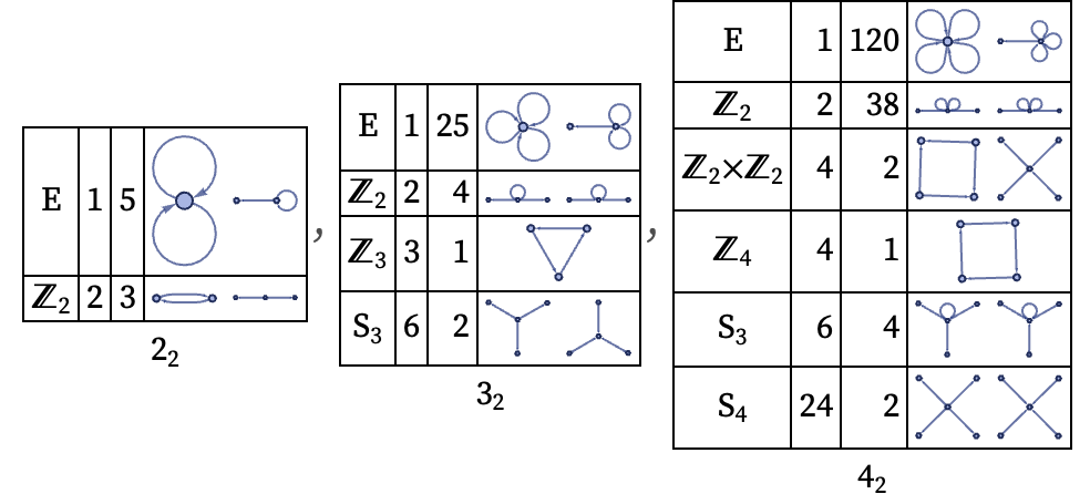
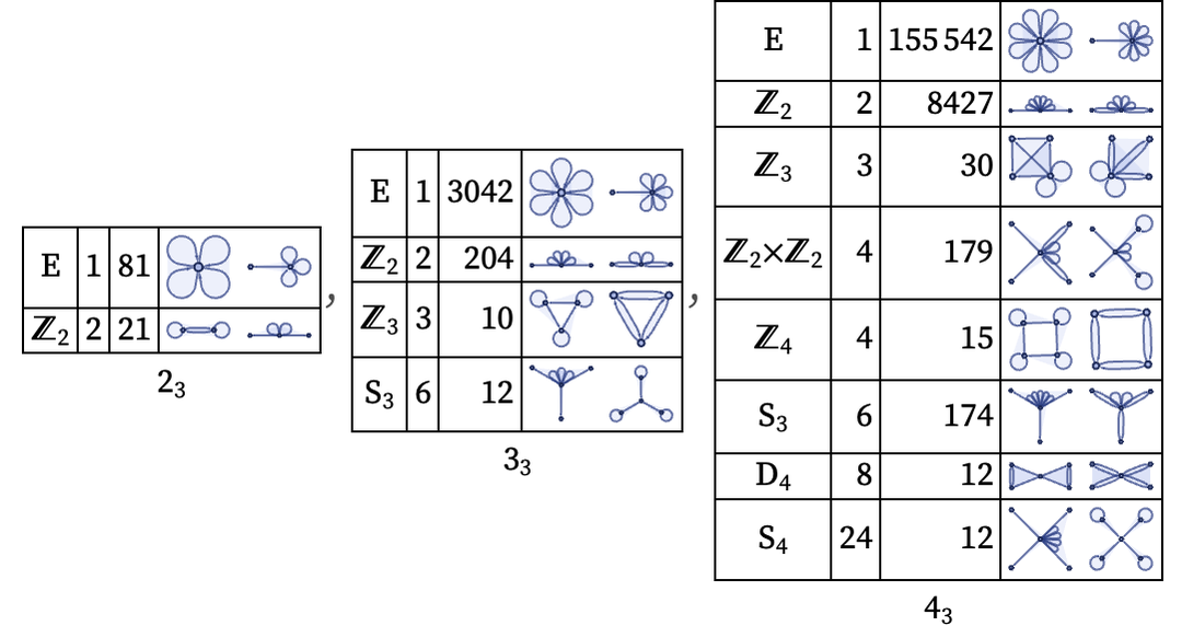
Here are automorphism groups for binary and ternary hypergraphs with various signatures. In each case the group order is included, as are a couple of sample hypergraphs:


If the right-hand side of a rule has at least as high a symmetry as the left-hand side, then any possible permutation of matches of elements will lead to the same result—which means that the same update will occur, and the only consequence will be a potential change in path weightings in the multiway graph.
But if the right-hand side of the rule has lower symmetry than the left-hand side (i.e. its automorphism group is a proper subgroup), then different permutations of matches can lead to different outcomes, on different branches of the multiway system. It may still nevertheless be the case that some permutations will lead to identical outcomes—and this will happen whenever the canonical form of the rule is the same after a permutation of the elements on the left-hand side (cf. [87]).
Thus for example the rule
is invariant under any of the permutations
of the elements corresponding to {x, y, z}. Note that the permutations that appear here do not form a group. To compose multiple such transformations one must take account of relabeling on the right-hand side as well as the left-hand side.
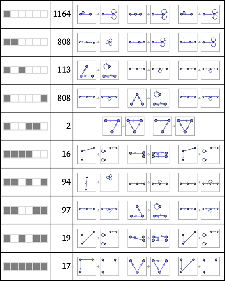
For the 3138 22 32 rules that involve 3 elements on the left, the following lists the 10 of 64 subsets of the 6 possible permutations that occur:

In a sense, we can characterize the local symmetry of a rule by determining what permutations of inputs it leaves invariant. But we can do this not only for a single update, but for a sequence of multiple updates. In effect, all we have to do is to form a power of the rule, and then apply the same procedure as above.
There are several ways to define a notion of powers (or in general, products) of rules. As one example, we can consider situations in which a rule is applied repeatedly to an overlapping set of elements—so that in effect the successive rule applications are causally connected.
In this case—much as we did for testing total causal invariance—we need to work out the unifications of the possible initial conditions. Then we effectively just need to trace the multiway evolution from each of these unified initial conditions.
Consider for example the rule:
The “square” of this rule is:

And its cube is:

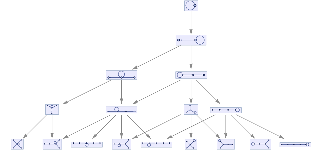
The multiway graph for the original rule after 4 updates is:

The “square” of the rule generates the same states in only 2 updates:

We can use the same approach to find the “square” of a rule like:
The result is:

Using this for actual evolution gives the result:

And now that we can compute the power of a rule, we have a way to compute the effective symmetry for multiple updates according to a rule. In general, after t updates we will end up with a collection of permutations of variables that leave the effective “power rule” invariant.
But if we now consider increasingly large values of t, we can ask whether the collections of permutations we get somehow converge to a definite limit. In direct analogy to the way that our hypergraphs can limit to manifolds, we may wonder whether these collections of permutations could limit to a Lie group (cf. [88]).
As a simple example, say that the permutations are of length n, but of the n! possibilities, we only have the n cyclic permutations, say for n = 4:
As n ∞ we can consider this to limit to the Lie group U(1), corresponding to rotations by any angle θ on a circle.
It is not so clear [89][90] how to deal in more generality with collections of permutations, although one could imagine an analog of a manifold reconstruction procedure. To get an idea of how this might work, consider the inverse problem of approximating a Lie group by permutations. (Note that things would be much more straightforward if we could build up matrix representations, but this is not the setup we have.)
In some cases, there are definite known finite subgroups of Lie groups—such as the icosahedral group A5 as a subset of the 3D rotation group SO(3). In such cases one can then explicitly consider the permutation representation of the finite group. It is also possible to imagine just taking a lattice (or perhaps some more general structure of the kind that might be used in symbolic dynamics [91][92]) and applying random elements of a particular Lie group to it, then in each case recording the transformation of lattice points that this yields. Typically these transformations will not be permutations, but it may be possible to approximate them as such. By inverting this kind of procedure, one can imagine potentially being able to go from a collection of permutations to an approximating Lie group.
 download pdf
  ARXIV
ARXIV peer review