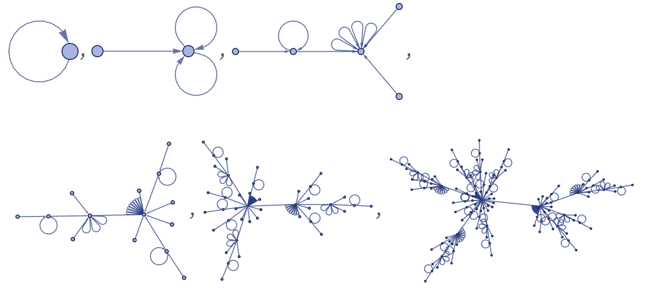
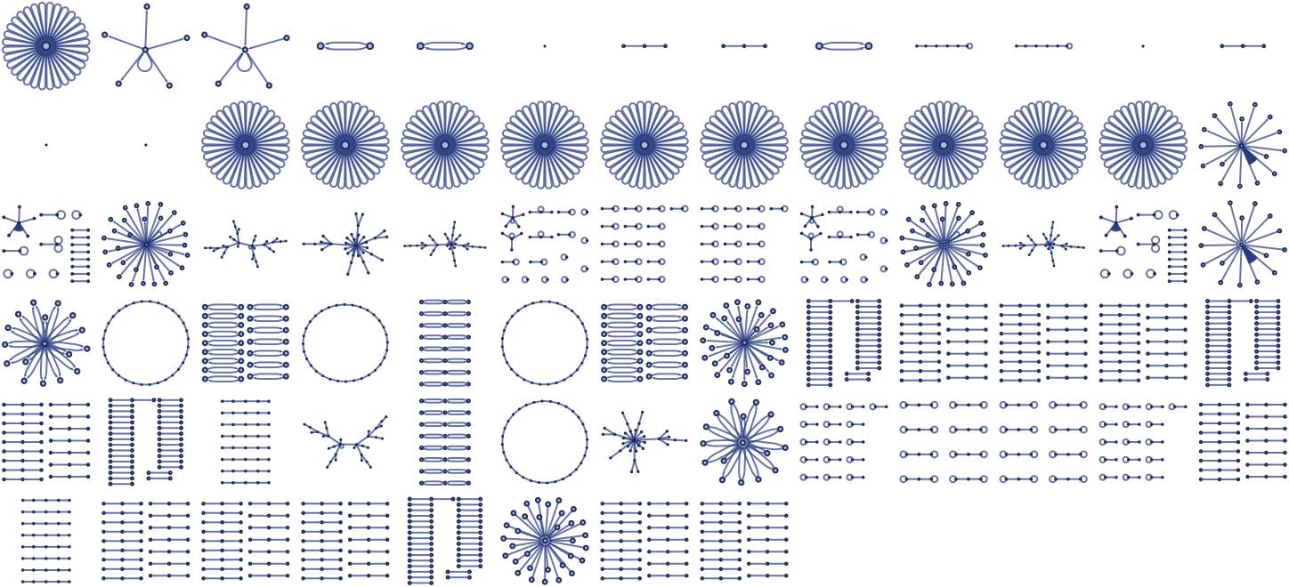
There are 73 inequivalent left-connected 12 22 rules, but none lead to structures more complex than trees. Starting each from a single self-loop, the results after 5 steps are (note that even a connected rule like {{x,y}}→{{x,z},{z,x}} can give a disconnected result):
GraphicsGrid[
Partition[
With[{ru =
ResourceFunction[
"EnumerateWolframModelRules"][{{1, 2}} -> {{2, 2}}]},
ParallelMap[
ResourceFunction["WolframModelPlot"][
ResourceFunction["WolframModel"][#, {{0, 0}}, 5, "FinalState"],
ImageSize -> Tiny] &, ru]], UpTo[13]], ImageSize -> Full]
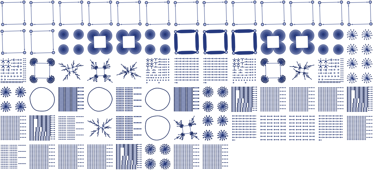
With an initial condition consisting of a square graph, the following very similar results are obtained:
GraphicsGrid[
Partition[
With[{ru =
ResourceFunction[
"EnumerateWolframModelRules"][{{1, 2}} -> {{2, 2}}]},
ParallelMap[
ResourceFunction["WolframModelPlot"][
ResourceFunction[
"WolframModel"][#, {{1, 2}, {2, 3}, {3, 4}, {4, 1}}, 5,
"FinalState"], ImageSize -> Tiny] &, ru]], UpTo[13]],
ImageSize -> Full]
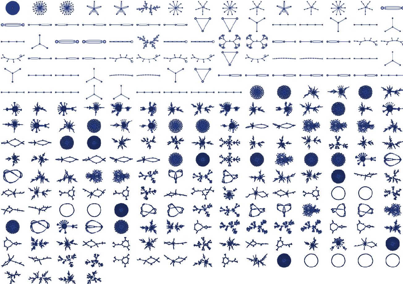
There are 506 inequivalent left-connected 12 32 rules. Running all these rules for 5 steps starting from a single self-loop, and keeping only distinct connected results, one gets (note that similar-looking results can differ in small-scale details):
Module[{rules =
ResourceFunction[
"EnumerateWolframModelRules"][{{1, 2}} -> {{3, 2}}], res},
res = ParallelMap[
ResourceFunction["WolframModel"][#, {{0, 0}}, 5, "FinalState"] &,
rules]; GraphicsGrid[
Partition[
ResourceFunction["WolframModelPlot"] /@
DeleteDuplicates[
Select[res, ConnectedGraphQ[Graph[UndirectedEdge @@@ #]] &]],
UpTo[15]], ImageSize -> Full]]
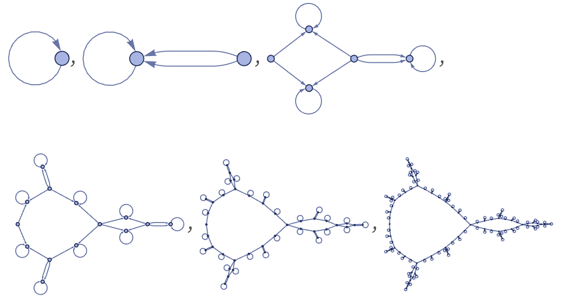
Several distinct classes of behavior are visible. Beyond simple lines, loops, trees and radial “bursts”, there are nested (“cactus-like”) graphs such as
ResourceFunction["WolframModelPlot"][#, "MaxImageSize" -> 180] & /@
ResourceFunction[
"WolframModel"][{{x, y}} -> {{x, z}, {y, z}, {z, z}}, {{1, 1}}, 5,
"StatesList"]
obtained from the rule:
{{x, y}} -> {{z, z}, {x, z}, {y, z}}
RulePlot[ResourceFunction[
"WolframModel"][{{x, y}} -> {{z, z}, {x, z}, {y, z}}]]
The only slightly different rule
{{x, y}} -> {{x, x}, {x, y}, {z, x}}
RulePlot[ResourceFunction[
"WolframModel"][{{x, y}} -> {{x, x}, {x, y}, {z, x}}]]
gives a rather different structure:
ResourceFunction[
"WolframModel"][{{x, y}} -> {{x, x}, {x, y}, {z, x}}, {{1,
1}}, 5, "StatesPlotsList"]
A layered rendering makes the behavior slightly clearer:
LayeredGraphPlot[Graph[Rule @@@ #], Bottom, AspectRatio -> 1,
VertexStyle ->
ResourceFunction["WolframPhysicsProjectStyleData"]["SpatialGraph",
"VertexStyle"],
EdgeStyle ->
ResourceFunction["WolframPhysicsProjectStyleData"]["SpatialGraph",
"EdgeLineStyle"]] & /@
ResourceFunction[
"WolframModel"][{{x, y}} -> {{x, x}, {x, y}, {z, x}}, {{1, 1}}, 5,
"StatesList"]
Another notable rule similar to one we saw in the previous section is:
{{x, y}} -> {{x, z}, {x, z}, {z, y}}
RulePlot[ResourceFunction[
"WolframModel"][{{x, y}} -> {{x, z}, {x, z}, {z, y}}]]
From a single edge this gives:
ResourceFunction[
"WolframModel"][{{x, y}} -> {{x, z}, {x, z}, {z, y}}, {{1,
2}}, 5, "StatesPlotsList"]
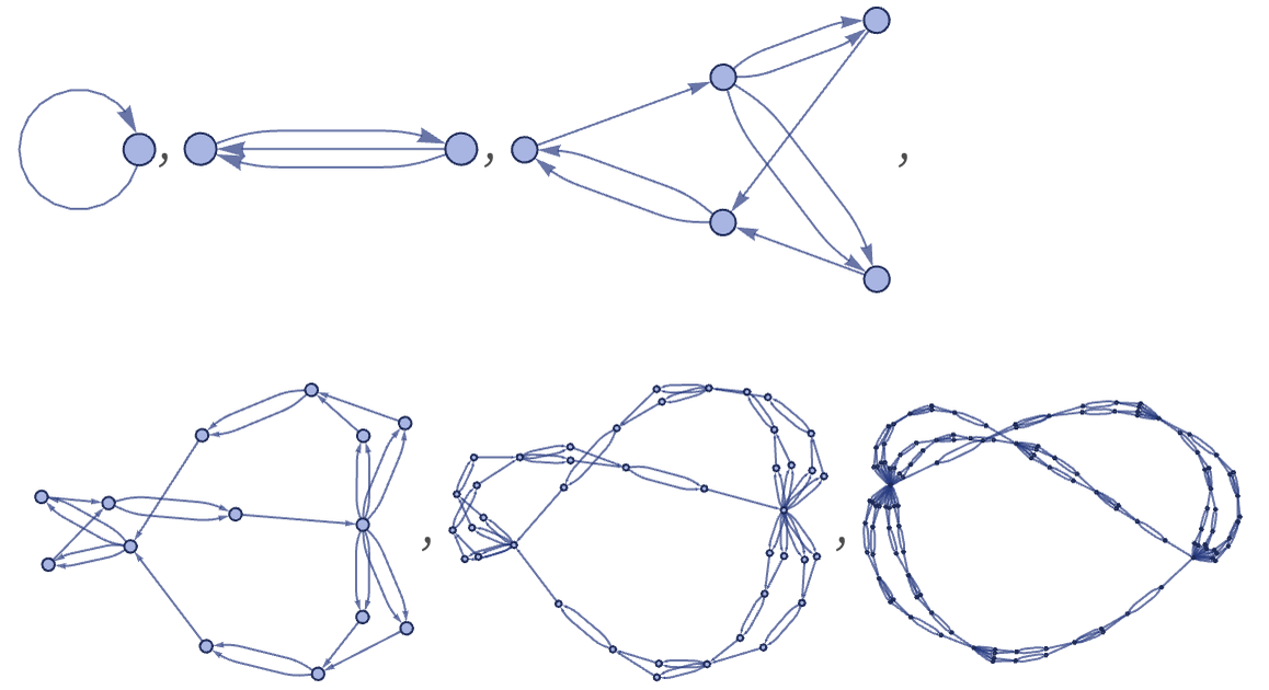
Starting from a single self-loop gives a more complex topological structure (and copies of this structure appear when the initial condition is more complex):
ResourceFunction[
"WolframModel"][{{x, y}} -> {{x, z}, {x, z}, {z, y}}, {{1, 1}},
5]["StatesPlotsList", "MaxImageSize" -> 180]
Another notable 12 22 rule is
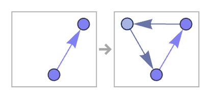
{{x, y}} -> {{x, y}, {y, z}, {z, x}}
RulePlot[ResourceFunction[
"WolframModel"][{{x, y}} -> {{x, y}, {y, z}, {z, x}}]]
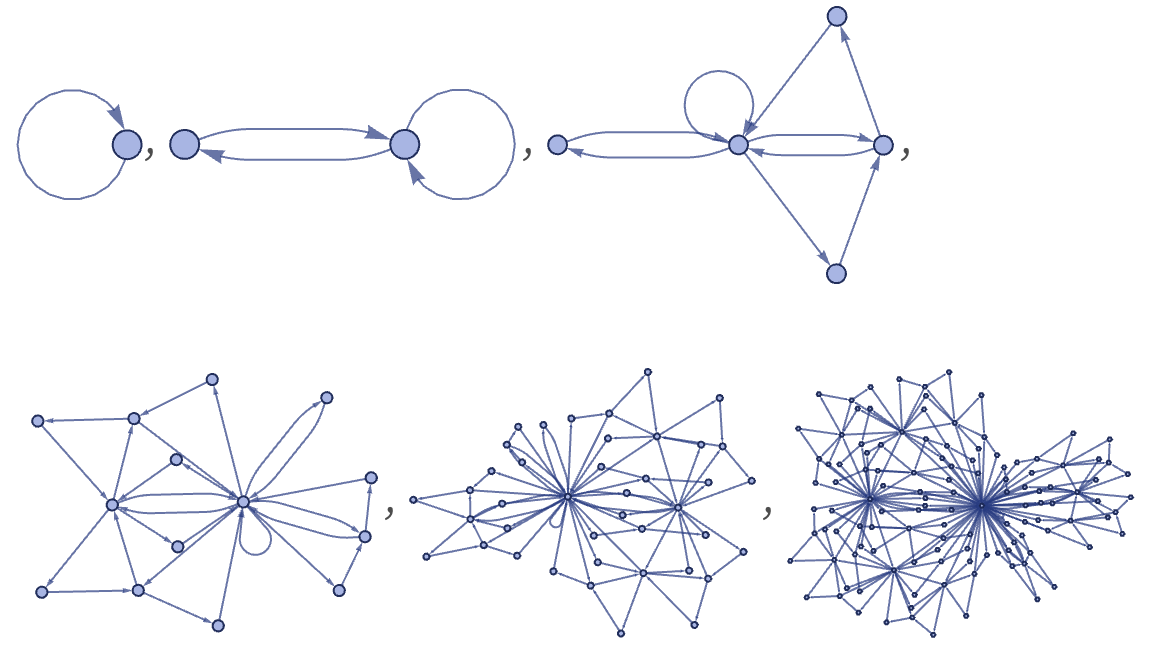
which produces an elaborately filled-in structure:
ResourceFunction[
"WolframModel"][{{x, y}} -> {{x, y}, {y, z}, {z, x}}, {{1, 1}},
5]["StatesPlotsList", "MaxImageSize" -> 180]
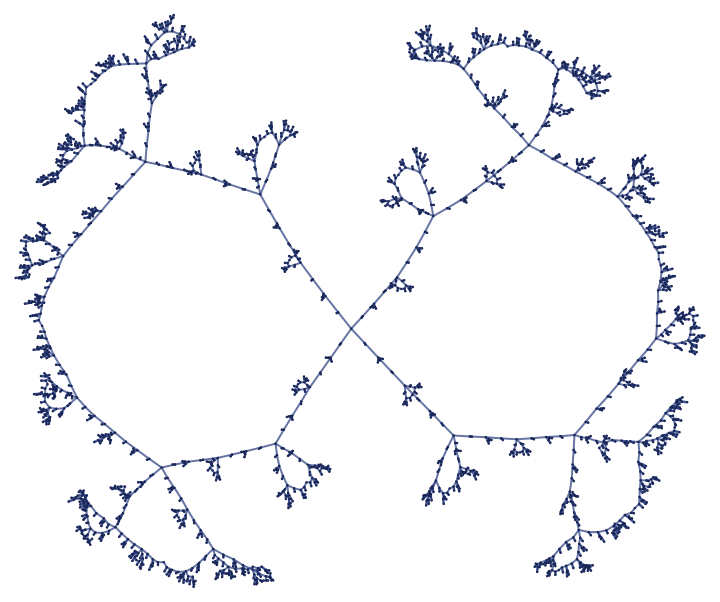
After 8 steps, the structure has the form:
GraphPlot[
Rule @@@ ResourceFunction[
"WolframModel"][{{x, y}} -> {{x, y}, {y, z}, {z, x}}, {{1, 1}}, 8,
"FinalState"],
VertexStyle ->
ResourceFunction["WolframPhysicsProjectStyleData"]["SpatialGraph",
"VertexStyle"],
EdgeStyle ->
ResourceFunction["WolframPhysicsProjectStyleData"]["SpatialGraph",
"EdgeLineStyle"]]
After t steps, there are 3t–1 nodes, and edges. The graph diameter is 2t – 1 if directions of edges are taken into account, and t – 1 if they are not. The maximum degree of any vertex is 2t—and all vertices have degrees of the form 2s, with the number of vertices of degree 2s being proportional to 3t–s.
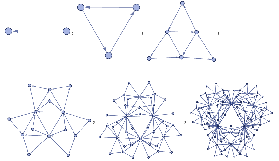
Starting from a single edge makes it slightly easier to understand what is going on:
ResourceFunction[
"WolframModel"][{{x, y}} -> {{x, y}, {y, z}, {z, x}}, {{1,
2}}, 5, "StatesPlotsList"]
As the rule indicates, every edge of every triangle “sprouts” a new triangle at every step, in effect producing a sequence of “frills upon frills”. But even though this may seem complicated, the whole structure basically corresponds just to a ternary tree in which each node is replaced by a triangle:
GraphicsRow[
Table[TreePlot[
KaryTree[Sum[3^i, {i, 0, n}], 3,
VertexStyle ->
ResourceFunction["WolframPhysicsProjectStyleData"][
"SpatialGraph", "VertexStyle"],
EdgeStyle ->
ResourceFunction["WolframPhysicsProjectStyleData"][
"SpatialGraph", "EdgeLineStyle"]], Center], {n, 1, 5}]]
Starting from a single self-loop, all 12 32 rules give after n steps a number of relations that is either constant, or goes like 2t – 1, 2t – 1 or 3t–1.
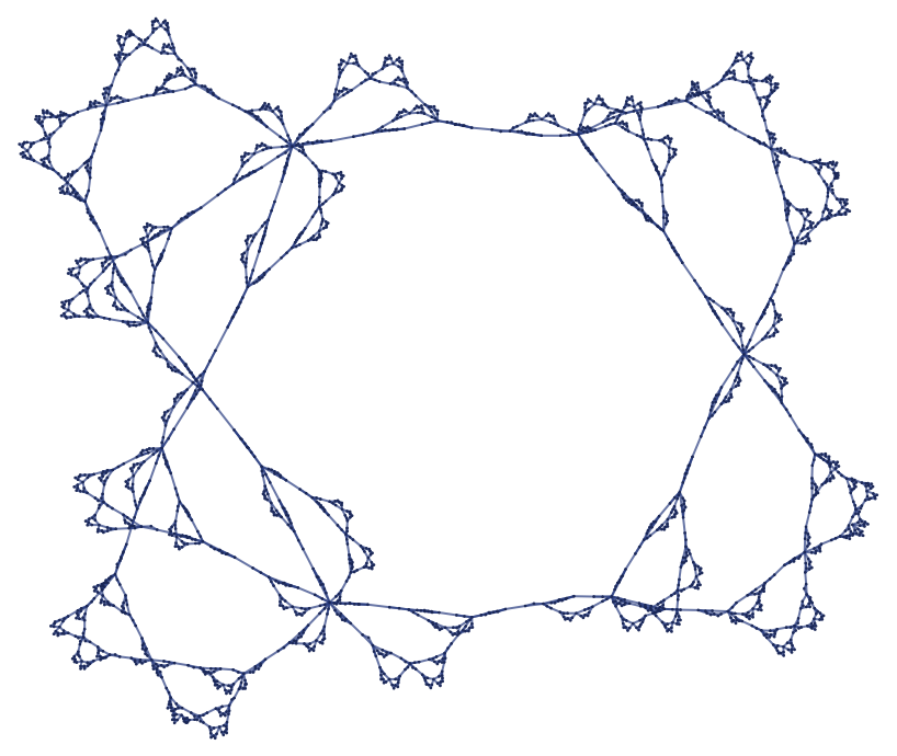
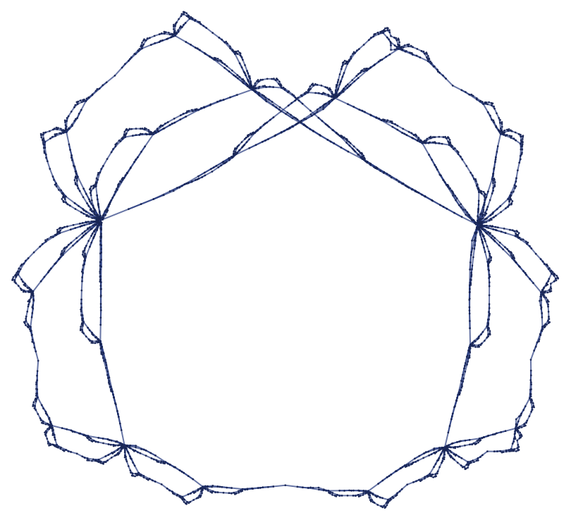
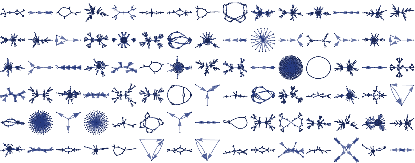
For 12 42, there are 3740 distinct left-connected rules. As suggested by the random cases below, their behavior is typically similar to 12 32 rules, though the forms obtained can be somewhat more elaborate:
CloudGet["https://wolfr.am/KWZib4Im"]
For example, the rule
{{x, y}} -> {{y, z}, {y, z}, {z, y}, {z, x}}
RulePlot[ResourceFunction[
"WolframModel"][{{x, y}} -> {{y, z}, {y, z}, {z, y}, {z, x}}]]
gives the following:
ResourceFunction["WolframModelPlot"][#, "MaxImageSize" -> 100] & /@
ResourceFunction[
"WolframModel"][{{x, y}} -> {{y, z}, {y, z}, {z, y}, {z, x}}, {{0,
0}}, 5, "StatesList"]
The rule
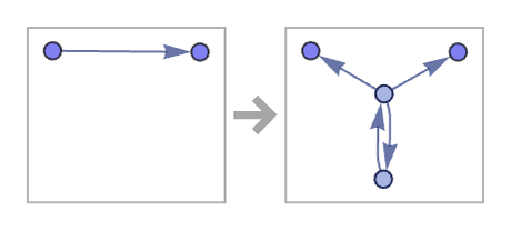
{{x, y}} -> {{z, w}, {w, z}, {z, x}, {z, y}}
RulePlot[ResourceFunction[
"WolframModel"][{{x, y}} -> {{z, w}, {w, z}, {z, x}, {z, y}}]]
gives a nested form:
ResourceFunction["WolframModelPlot"][#, "MaxImageSize" -> 100] & /@
ResourceFunction[
"WolframModel"][{{1, 2}} -> {{3, 4}, {4, 3}, {3, 1}, {3, 2}}, {{0,
0}}, 5, "StatesList"]
ResourceFunction[
"WolframModel"][{{x, y}} -> {{z, w}, {w, z}, {z, x}, {z, y}}, {{0,
0}}, 6, "FinalStatePlot"]
The rule
{{x, y}} -> {{y, z}, {y, w}, {z, w}, {z, x}}
RulePlot[ResourceFunction[
"WolframModel"][{{x, y}} -> {{y, z}, {y, w}, {z, w}, {z, x}}]]
gives
ResourceFunction["WolframModelPlot"][#, "MaxImageSize" -> 100] & /@
ResourceFunction[
"WolframModel"][{{x, y}} -> {{y, z}, {y, w}, {z, w}, {z, x}}, {{0,
0}}, 5, "StatesList"]
ResourceFunction[
"WolframModel"][{{x, y}} -> {{y, z}, {y, w}, {z, w}, {z, x}}, {{0,
0}}, 6, "FinalStatePlot"]
while the similar rule
{{x, y}} -> {{x, z}, {x, w}, {z, w}, {z, y}}
RulePlot[ResourceFunction[
"WolframModel"][{{x, y}} -> {{x, z}, {x, w}, {z, w}, {z, y}}]]
gives:
ResourceFunction["WolframModelPlot"][#, "MaxImageSize" -> 100] & /@
ResourceFunction[
"WolframModel"][{{x, y}} -> {{x, z}, {x, w}, {z, w}, {z, y}}, {{0,
0}}, 5, "StatesList"]
ResourceFunction[
"WolframModel"][{{x, y}} -> {{x, z}, {x, w}, {z, w}, {z, y}}, {{0,
0}}, 6, "FinalStatePlot"]
Successive steps in effect just fill in this shape, which seems somewhat irregular when rendered in 2D, but appears more regular if rendered in 3D.
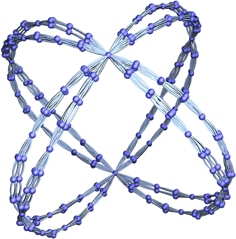
Another rule with a simple structure when rendered in 3D is
{{x, y}} -> {{y, z}, {y, z}, {z, x}, {z, x}}
RulePlot[ResourceFunction[
"WolframModel"][{{x, y}} -> {{y, z}, {y, z}, {z, x}, {z, x}}]]
which yields:
ResourceFunction["WolframModelPlot"][#, "MaxImageSize" -> 100] & /@
ResourceFunction[
"WolframModel"][{{1, 2}} -> {{2, 3}, {2, 3}, {3, 1}, {3, 1}}, {{0,
0}}, 5, "StatesList"]
GraphPlot3D[
Rule @@@ ResourceFunction[
"WolframModel"][{{1, 2}} -> {{2, 3}, {2, 3}, {3, 1}, {3, 1}}, {{0,
0}}, 5, "FinalState"],
VertexStyle ->
ResourceFunction["WolframPhysicsProjectStyleData"]["SpatialGraph3D",
"VertexStyle"],
EdgeStyle ->
ResourceFunction["WolframPhysicsProjectStyleData"]["SpatialGraph3D",
"EdgeLineStyle"]]
The outputs from 12 42 rules all grow either linearly (for example, like 3t – 2), or exponentially, asymptotically like 2t, 3t or 4t. The number of relations after t steps is always given by a linear recurrence relation; for the rule {{x,x}}{{x,x},{x,x},{x,y},{x,y}} the recurrence is f[t]=3f[t–1]–2f[t–2] (with f[1]=1, f[2]=4), giving size .